MIKE FM Ensemble modelling

The two main reasons for creating an ensemble model are:

1. Uncertainty quantification. To evaluate the uncertainty of your model including how uncertainties correlate across space and variables.

2. Data assimilation with the Ensemble Kalman Filter (EnKF). An ensemble is used to estimate the model error covariance $P$ allowing assimilation with the Kalman update equation.

The ensemble of model states in a MIKE FM DA model is created by stochastically perturbing model forcings, initial conditions or model parameters.

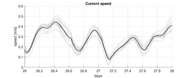A timeseries of current speed from an ensemble model.

In MIKE FM, these perturbations are called model errors and both for uncertainty quantification and assimilation with the EnKF, it is crucial to have a “good” description of model errors which gives a “natural” variability of the ensemble model. If, as an example, the main source of a model's uncertainty is the position of salinity gradients, then a realistic perturbation of the model will not be obtained by perturbing the wind input. It is the responsibility of the modeller to provide a good and realistic description of model errors.

This page focuses on explaining how ensemble modelling works in MIKE FM. See the reference for how to specify the MODEL_ERROR pfs section.

Terminology

Term	Description
Ensemble	A collection of model realizations
Member	A single model realization in an ensemble
Model error	Perturbation of model quantity (e.g. change of a water level boundary)
Model error model	The "model" (or "error formulation") describing the discretization, correlation structure, and time propagation of the model error

Why is the model wrong?

The typical sources of uncertainty in MIKE FM models are:

a. Initial condition errors (initial state)

b. Forcing errors (data from outside) such as boundary errors, meteorological forcings (e.g. wind)

c. Model formulation errors such as discretization, equations and parameterizations (the model itself)

d. Parameter errors (settings made by the modeller) (e.g. bottom friction)

The DA module supports the description of errors in forcings (b) and in selected parameters (d). Perturbation of initial conditions (a) can be handled by the modeller as a pre-processing step. The DA module does not support internal model errors (c) originating from the governing equations, in-accurate parameterizations or too coarse model resolution.

Model errors

A MIKE FM model can have any number of model errors. Each model error is normally distributed with zero mean and is represented by a (state) vector of values which may change over time. Each model error modulates some MIKE FM quantity (e.g. a wind forcing) and have its own discretization and propagation model. Each ensemble member is modulated differently by the model errors which hereby provides a variation of model realizations.

Model error type

Any type of model error needs to be related to the underlying MIKE FM model. In some cases, this is done simply be specifying the type of the model error in other cases the user needs to supply more information e.g. the id of a FM quantity. A "water level boundary error" is an example of a model error type.

Model error modelling (error formulation)

Each model error needs to be formulated by specifying the

• Amplitude and perturbation type (additive, multiplicative, ...)
• Temporal propagation including initialization
• Spatial discretization (horizontal and vertical)
• Spatial correlation (horizontal and vertical)

Not all items are relevant for all model errors, e.g., no spatial discretization or correlation description is needed for global parameters or 0D sources.

Amplitude and perturbation type

The most basic specification of the model error formulation is the perturbation type (e.g. additive or multiplicative) and the amplitude of the error specified as a standard deviation “st_dev” of the Gaussian error process. Note that the error process is assumed to have zero mean. It is furthermore possible to provide minimum and maximum values e.g. to ensure physically realistic values.

The two main categories of perturbation_types are available:

• additive (default)
• multiplicative

A number of variants exists e.g. ensuring non-negativity or boundedness of the perturbed quantity. See amplitude-and-perturbation-type specification for details.

An additive perturbation of the quantity $x$ consists of the following manipulation:

$$x := x + \varepsilon$$

The amplitude (st_dev) of the error $\varepsilon$ will therefore be in the same unit as the FM quantity being modified $x$. For a water level boundary error, as example, the error amplitude expressed by st_dev will be in meters.

Multiplicative perturbations take the following form:

$$x := x (1 + \varepsilon)$$

The st_dev will in such cases be relative. If we wish to have a 10% variation in the water level boundary error the st_dev should be $0.1$.

Temporal propagation

In most cases, the model error will have a temporal propagation model associated. The following “propagation_type”s are available

• AR(1) – first order auto-regressive process (default)
• persistence – i.e. no temporal propagation
• whitenoise

Please experiment with the AR(1) app to get a better understanding of auto-regressive processes and the associated parameters.

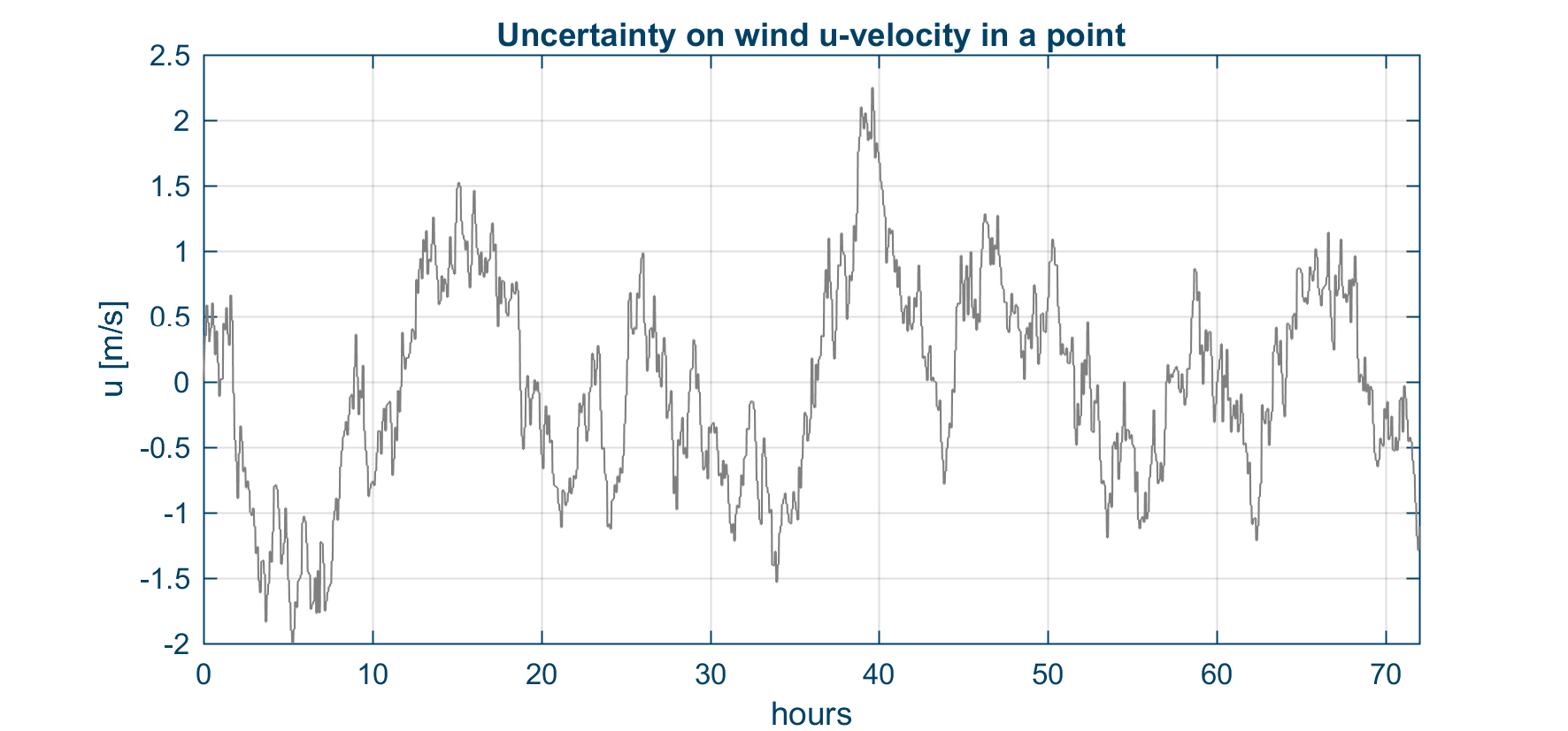The graph shows an example of an AR(1) process describing wind variability in a point.

Spatial discretization

If the model error has a spatial extent (e.g. a boundary or wind error) it needs to be discretized in space. The discretization will typically be coarser than the resolution of the corresponding MIKE FM quantity (e.g. the model mesh). The DA engine will perform a (bi-) linear interpolation from the discretized error on to the model quantity before the actual perturbation is done.

Currently three options exist for horizontal discretization of model errors:

• Type 0: Constant
• Type 1: Linear
• Type 2: Equidistant grid

This may be extended with an unstructured type in the future.

Discretization of boundary errors

Model errors on open boundaries can be either constant (type 0), or discretized linearly by model error points in the endpoints (type 1) or on a regular grid (type 2).

Connected open boundaries should be modelled as a group of boundary segments (a single model error). The discretization types then hold for each segment such that it will be piecewise constant (type 0), piecewise linear (type 1) or on regular grid (type 2).

See an example below.

Discretization of 2d errors

Model errors covering the 2d domain like the wind error can be constant in space (type 0) or discretized on a regular 2d grid (type 2). Type 1 is a special case of type 2 with only the corner nodes of the overset grid.

See an example below.

Spatial correlation

The spatially distributed errors are in most cases correlated in space. Internally in the code the correlation is described by a covariance matrix Q which describes how the errors co-vary across the domain. The user can control this both indirectly by the horizontal discretization (see above section) and directly by specifying a horizontal correlation length scale (and function). A typical value for the horizontal correlation could be 5-10 times larger than the horizontal grid spacing. The specified correlation length should reflect the dynamics of the corresponding error, but our best guess of this value will often be the correlation length of the quantity itself (e.g. 300km for the wind).

Please experiment with the horizontal correlation app to get a better understanding of correlated errors on an equidistant grid.

Example 1: Water level boundary condition error

Consider a HD model in the domain shown on the below figure with a mesh with an average element side length of 8 km. The water level boundary consists of five sections (Norteast, North, West, South and Southeast).

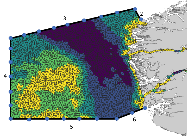
The boundary sections are connected and their perturbation should therefore be modelled with a single water level boundary error. The error could have the following specifications:

Property	Value	Comment
st_dev	0.04 m	The range of the water level is 1.1 m in this area.
perturbation_type	additive	The default choice
propagation_type	AR(1)	The default choice
half time	4 hours	Estimated from the temporal dynamics of the water levels
grid_spacing	50 km	Coarser than the model resolution of 8 km
spatial correlation	300 km	Based on correlation length of the water level in the model

Example 2: Wind error

Consider the same HD model as above. We can discretize the wind error over this domain on a regular grid with a spacing of approximately 100km as shown on the below figure.

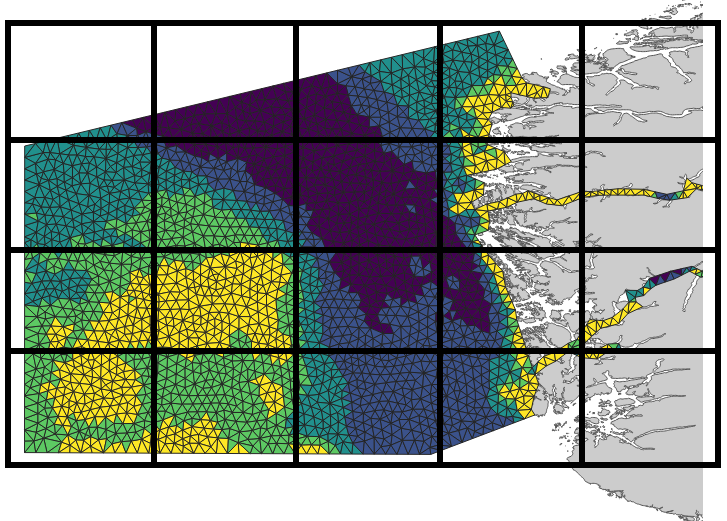
The wind error is actually 2 independent model errors: u-component and v-component errors.

Property	Value	Comment
st_dev	3.5 m/s	The range of values in the wind forcing is 30.
perturbation_type	additive	The default choice
propagation_type	AR(1)	The default choice
half time	3 hours	Estimated from the temporal dynamics of the wind
grid_spacing	100 km	Coarser than the model resolution of 8 km
spatial correlation	400 km	Based on correlation length of the forcing

List of model errors by FM module

As stated above, the specification of a model error consists of a) the FM specification and b) the error formulation.

Type of errors currently supported by the DA module:

Hydrodynamic module HD

• Boundary conditions
  • water level
  • velocity/flux
  • time shift
• Wind forcing
  • wind components
  • wind speed
  • wind phase (time shift)
• Parameters
  • bed_resistance_coefficient
  • bed_resistance

Temperature/salinity module TS

• Boundary conditions
  • temperature
  • salinity
  • time shift
• AD Source
  • concentration (salinity/temperature)
• Parameters
  • vertical_dispersion_coefficient
  • vertical_eddy_viscosity_coefficient
  • light_extinction

Transport module TR

• Boundary conditions
  • AD component
  • time shift
• AD Source
  • concentration (AD component)
• Parameters
  • vertical_dispersion_coefficient
  • vertical_eddy_viscosity_coefficient
  • decay rate

Mud Transport module MT

• Boundary conditions
  • fraction concentration
  • time shift
• AD Source
  • concentration (fraction)
• Parameters
  • vertical_dispersion_coefficient
  • vertical_eddy_viscosity_coefficient
  • settling_velocity
  • settling_velocity_coefficient
  • deposition_critical_shear_stress
  • erosion_critical_shear_stress
  • bottom roughness
  • dredger rate
  • dredger spill
  • dredger phase

Ecolab module EL

• Boundary conditions
  • state_variable concentration
  • time shift
• AD Source
  • concentration (state_variable)
• Parameters
  • vertical_dispersion_coefficient
  • vertical_eddy_viscosity_coefficient
  • EL Constants
  • EL state_variable
  • EL forcing

Spectral wave module SW

• Boundary conditions
  • time shift
  • wave height scaling (scaling of total energy)
  • wave period shift
  • wave direction shift
• Wind forcing
  • wind components
  • wind speed
  • wind phase (time shift)
• Parameters
  • background_Charnock_parameter
  • wind_non_dimensional_growth
  • wind_corr_friction_velocity_CAP
  • whitecapping_dissipation_cdiss
  • whitecapping_dissipation_delta
  • whitecapping_cds_sat
  • Nikuradse_roughness

Ensemble forcings

Since MIKE release 2022 update 1, an additional method for creating an ensemble has been available: ENSEMBLE_FORCINGS. An ensemble forcing (e.g. ensemble wind from GFS or ECMWF) can be used to force your ensemble FM model by specifying ensemble items for each of the forcing variables (e.g. wind speed and direction items).

See ENSEMBLE FORCINGS section for more information.

Available ensemble forcings per model

Module	forcing_type	Description
HD	wind	Typically given as pressure and u- and v-components as the wind
SW	wind	Typically given as speed and direction

See ENSEMBLE FORCINGS section for more about the specification.

Ensemble input and outputs

The state vector for all ensemble members can be outputted to disk in the ENSEMBLE_IO section. The same section can be used to specify ensemble input data to “hot start” an ensemble model.

The DIAGNOSTICS section is very useful for producing ensemble time series output for a specific variable in a specific point.