Examples

PFS examples containing the sections you need to add to your FM model are available for download:

• DA pfs minimal example
• DA pfs example for HD
• DA pfs example for TR
• DA pfs example for MT
• DA pfs example for EL
• DA pfs example for SW

Full runnable examples are also available for download:

• HD-DA example Oresund2D - see description below
• TR-DA example FunningsFjord - see description below
• MT-DA example TidalChannel - see description below
• MT-DA example Dredging in Harbor - see description below
• SW-DA example SouthernNorthSea - see description below

See also how to quickly create a new DA model.

HD

Oresund HD2D basic

This example (download files) shows how assimilation of two water level stations can improve the results of a 2D HD model significantly.

A. HD model

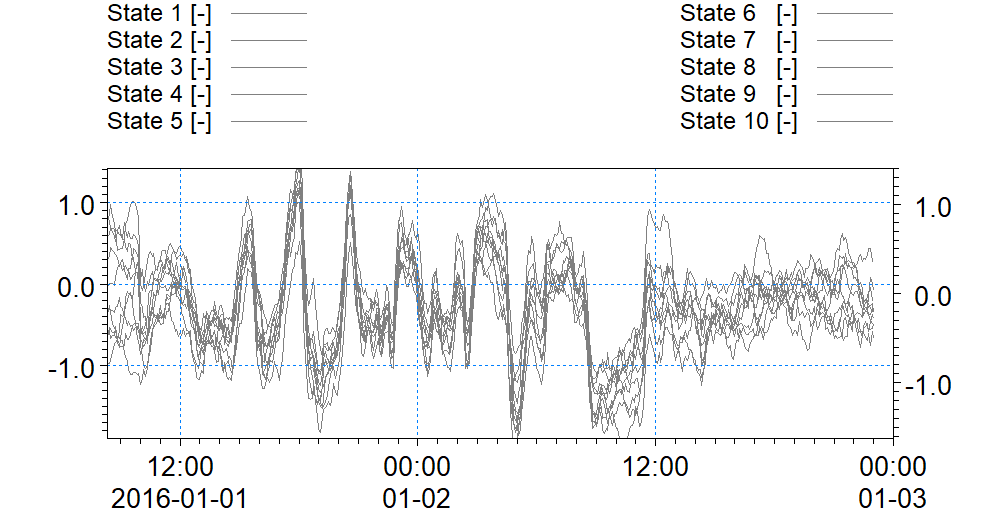
B. "Free5" Ensemble model without assimilation "Free run" with 5 ensemble members by perturbing the water level boundary conditions North and South

C. "EnKF10" Ensemble Kalman filter (EnKF) model with 10 ensemble members and same perturbation as in B; 2 water level stations are used for assimilation, 2 for validation

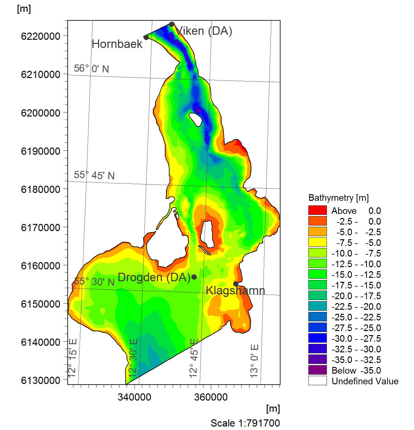Map showing the domain and observations for the OresundHD2D example.

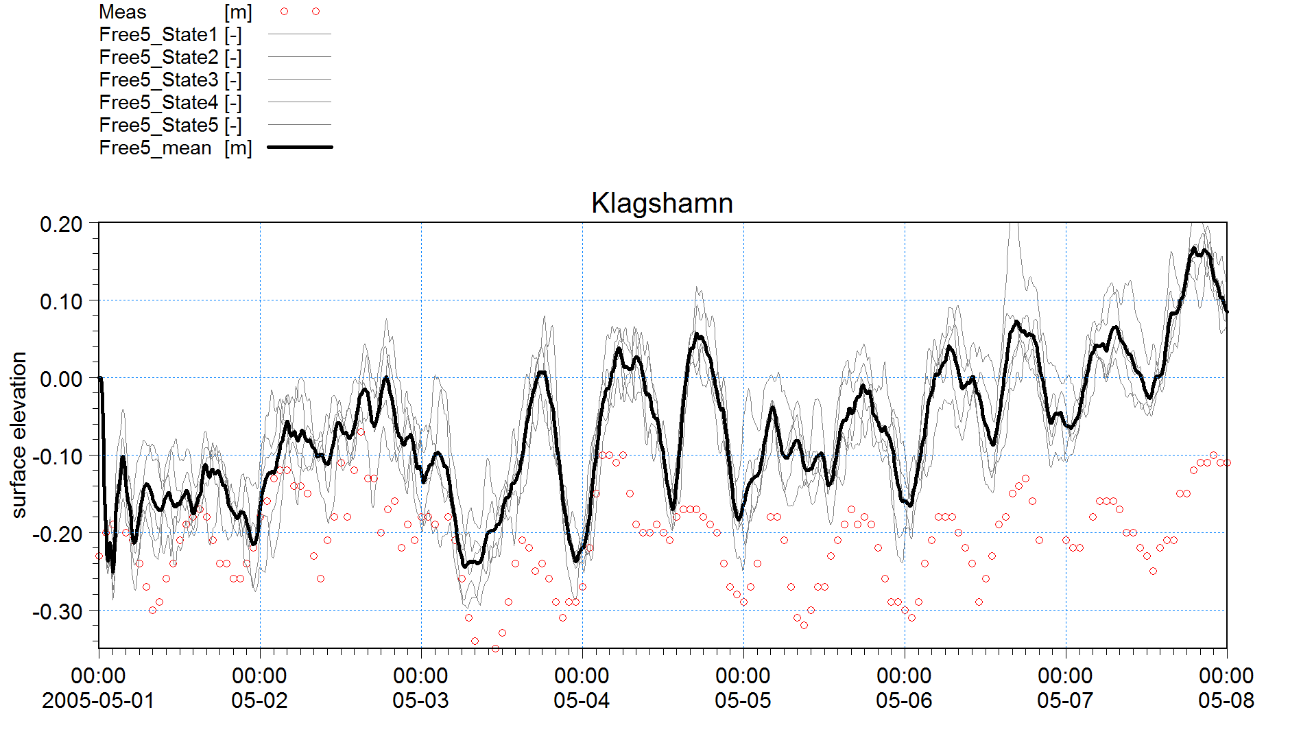Time series of the water level in Klagshamn for the Free5 ensemble run (without data assimilation).

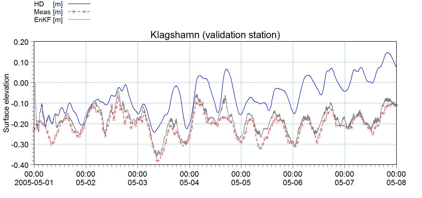Time series of the water level in Klagshamn for HD, Free5, and EnKF10.

TR

Funnings Fjord

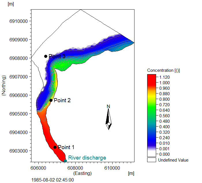
This transport module example (download files) features a Fjord system and discharge of some harmful substance from the river in the bottom of the Fjord. The hydrodynamics is driven by a tidal boundary condition and temporal varying wind field.

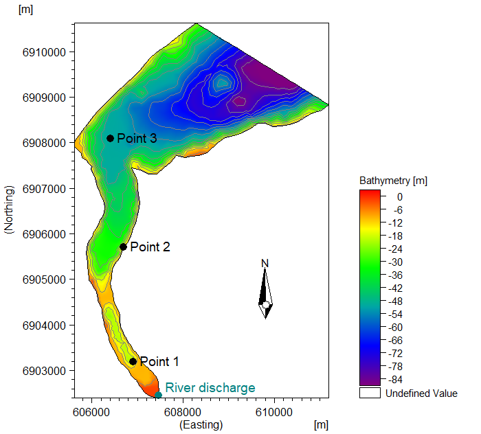
Model domain, bathymetry, and the three measurement points of the Funnings Fjord TR example.

The transport module is run decoupled and is hotstarted with the concentration shown in the below figure.

Initial tracer concentration shown on the map.

The example includes the following set-ups:

A. HD with decoupling output

B. TR decoupled without data assimilation

C. TR-DA free ensemble run with perturbation of the decay parameter and the source concentration

D. TR-DA EnKF run with the same perturbations and assimilation of concentration at Point 2

E. TR-DA Nudging run with assimilation of concentration at Point 2

The below time series show the concentrations for the different simulations at the point of assimilation (Point 2) and the validation point (Point 1).

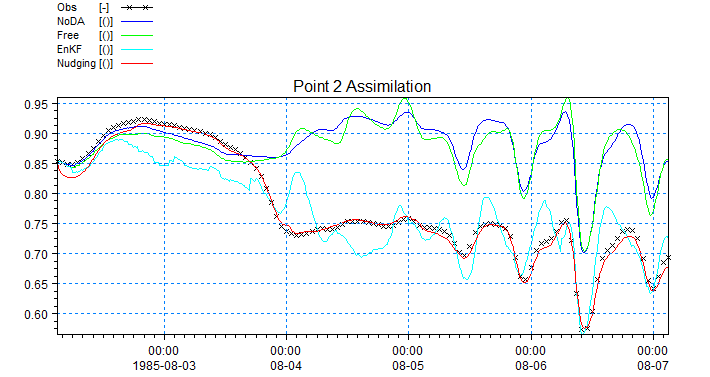
Time series showing tracer concentration in point of assimilation (point 2).

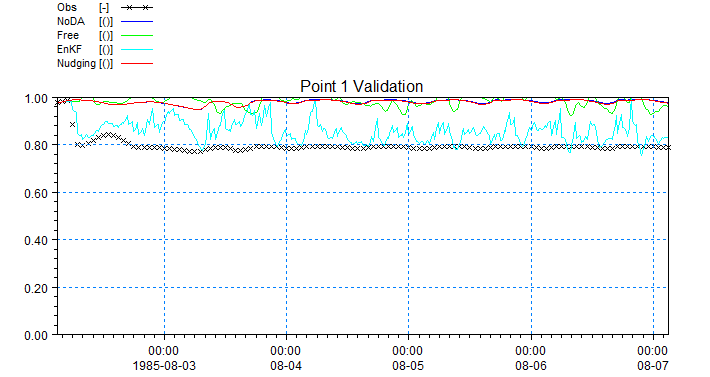
Time series showing tracer concentration in a validation point (point 1).

MT

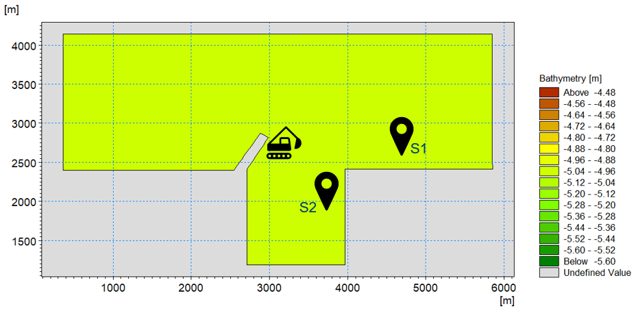
Tidal Channel

In this example (download files) a section of a tidal (oscillating current directions) channel is modelled. The objective is to use data assimilation to improve the model predicting the oscillating SSC levels occurring inside the channel. Three measurement points are assumed inside the channel which shall be used for data assimilation and validation of the model.

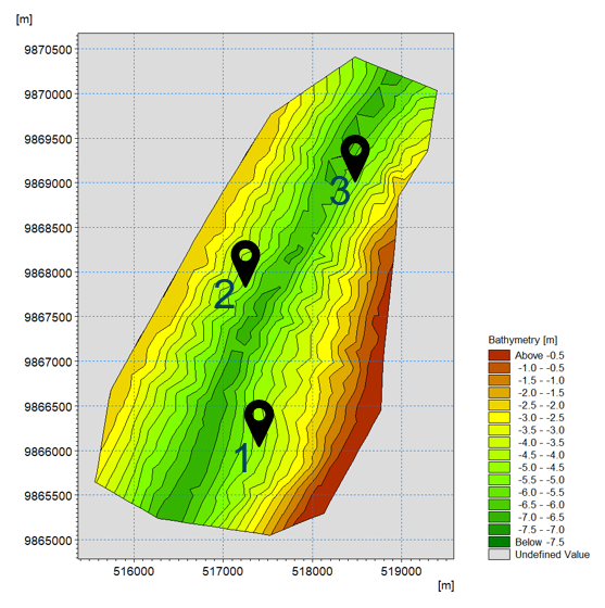
Model domain, bathymetry, and the three measurement points of the Tidal Channel example.

In order to simplify this exercise, the following assumptions are made:

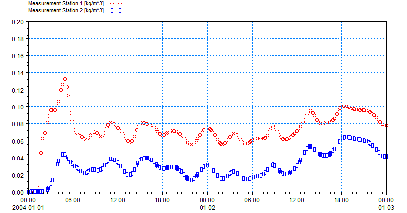
• Data on SSC levels from three measurement stations are available, and it is assumed that they contain an error with standard dev. Of 0.05 kg/m3

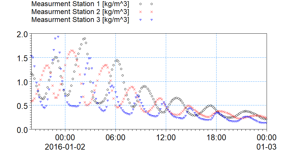Measured SSC levels at three stations shown on map in the above figure.

• The model runs in Decoupling mode, meaning that HD variables are set.
• The initial conditions for SSC levels and seabed are thickness of 1m. and SSC = 0.0 kg/m3.
• The SSC boundary condition at South is assumed zero gradient
• The SSC boundary condition at North is known, but with errors on both the value (with standard dev. of 0.5 kg/m3) and the phase (with standard dev. of 30 minutes)

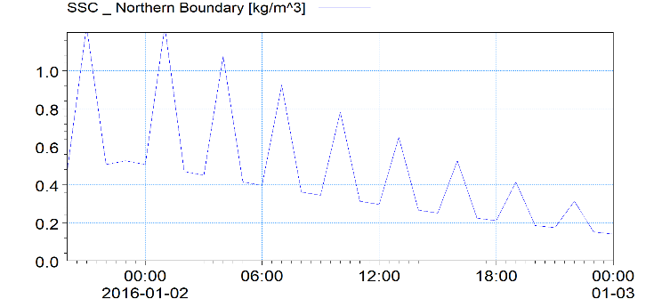
SSC boundary conditions at Northern open boundary.

• The sediment size is known but with an error, translated to an error on fall velocity (with standard deviation of 0.001 mm/s)

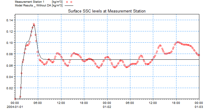
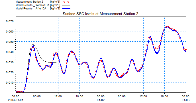
The model results without data assimilation are not satisfactory when comparing to the measurements. The figure below shows the model results in comparison with measured SSC levels at station 1. There are differences both in magnitude and phase.

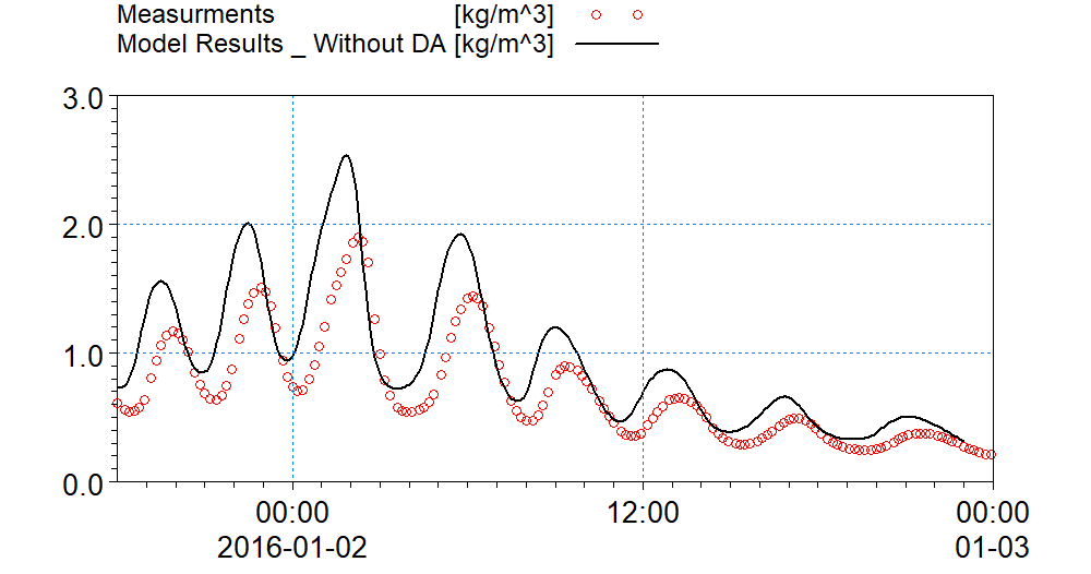Comparison between measured SSC levels and model results without data assimilation.

The data assimilation module is added to the pfs setup file. The number of ensemble members is set to 10, and the Ensemble Kalman Filter method (type=1) is chosen for assimilation.

[METHOD]
    type = 1
    ensemble_size = 10
    Rfactor_anomalies = 3
EndSect  // METHOD

The time step for beginning the ensemble modelling is set to 100, and the time step for applying data assimilation is set to 120. The data assimilation time steps are set to equal to the overall model time steps.

[TIME]
    start_time_step = 100
    start_time_step_assimilation = 120
    time_step_factor_assimilation = 1
EndSect  // TIME

Three different model errors are introduced in the data assimilation section:

1- Model error on SSC phase at Northern Boundary

[MODEL_ERROR_1]
    type = 'adbc'
    fraction_id = 1
    n_bounds = 1 
    bound_codes = 3
    is_phase_error = True
    [Error_Formulation] 
        st_dev = 1800
        minimum_value = -3600
        maximum_value = 3600
        perturbation_type = 'additive'
        propagation_type = 'AR(1)' 
        propagation_parameter = 18000
        initialization_type = 1
    EndSect
EndSect  // MODEL_ERROR_1

2- Model error on SSC magnitudes at northern boundary:

[MODEL_ERROR_2]
    type = 'adbc'
    fraction_id = 1
    n_bounds = 1 
    bound_codes = 3
    is_phase_error = False
    [Error_Formulation] 
        st_dev = 0.5
        perturbation_type = 'additive'
        propagation_type = 'AR(1)'
        propagation_parameter = 18000
        initialization_type = 1
    EndSect
EndSect  // MODEL_ERROR_2

3- Model error on settling velocity coefficient magnitude

[MODEL_ERROR_3]
    type = 'MT_parameter'
    parameter_name = 'settling_velocity_coefficient'  
    fraction_id = 1
    [ERROR_FORMULATION]
        st_dev = 0.00001
        perturbation_type = 'additive_non_negative'
        propagation_type = 'AR(1)'
        propagation_parameter = 72000
        initialization_type = 1
        horizontal_discretization_type = 0
    EndSect  // ERROR_FORMULATION
EndSect  // MODEL_ERROR_3

Notice that the “propagation_parameter” is related to the period in error generation (perturbation) function, and depending on the type of variable, the model behavior and the user’s experience be manipulated for getting better results.

The three measurement points are added to the measurement section. Two of the points (Stations 2 & 3) are set to be used for data assimilation, and the remaining point (Station 1) is set to be used as validation point.

[MEASUREMENTS]
    number_of_independent_measurements = 3
    [MEASUREMENT_1]
        name = 'point1'
        include = 2  //0= exclude , 1: assimilation , 2: validation
        measured_variable = 'MT%SSC_FRACTION_1'
        type = 1                  
        file_name = |..\obs\ssc_obs_points_2.dfs0|
        item_number = 1
        position = 516845.699320,  9866165.622750
        st_dev = 0.05
    EndSect  // MEASUREMENT_1

    [MEASUREMENT_2]
        name = 'point2'
        include = 1
        measured_variable = 'MT%SSC_FRACTION_1'
        type = 1                  
        file_name = |..\obs\ssc_obs_points_2.dfs0|
        item_number = 2
        position = 518073.702458, 9867178.725339
        st_dev = 0.05
    EndSect  // MEASUREMENT_2

    [MEASUREMENT_3]
        name = 'point3'
        include = 1
        measured_variable = 'MT%SSC_FRACTION_1'
        type = 1                  
        file_name = |..\obs\ssc_obs_points_2.dfs0|
        item_number = 3
        position = 518089.0524972, 9868990.029967
        st_dev = 0.05
    EndSect  // MEASUREMENT_3
EndSect  // MEASUREMENTS

In order to write out the error values created at each Model Error as a result of perturbations under data assimilation process, the “Ensemble_IO” output section can be activated. The type of files follows the nature of the model error. For example, the boundary error (error 2) is written out as dfs1 files because it's applied along the boundary. Phase errors are "time offsets" per input file and therefore dfs0. The parameter error (error 3) is written as dfs2 file because it’s been applied over the entire model domain. The resulting state of the model (which in this case are the SSC values and bed mass) will be written out as dfsu files. The “type” tells if it writes out the mean state, or all the ensemble members.

[ENSEMBLE_IO]     
    [INPUT]
        type = 0  // 0: not active, 1: Meanstate, 2: Ensemble   
    EndSect  // INPUT

    [OUTPUTS]
        number_of_outputs = 1
        [OUTPUT_1]
            type = 0  // 0: not active, 1: Meanstate, 2: Ensemble
            file_name_area = 'State_Area.dfsu'  
            file_name_err01_adbc = 'err01.dfs1'
            file_name_err02_adbc = 'err02.dfs1'
            file_name_moderr3_mtpar = 'err03.dfs2'
        EndSect  // OUTPUT_1
    EndSect // OUTPUTS
EndSect  // ENSEMBLE_IO

The “Diagnostic Output” writes out a state variable (SSC or bed mass) for all the ensemble members as well as their mean value. This can be done at the measurement points, or at any desirable point inside the domain.

[DIAGNOSTICS]
    [OUTPUTS]
        number_of_outputs = 4
        [OUTPUT_1]
            type = 1
            measurement_id = 1      
            file_name = 'diagnostics_meas1.dfs0'        
        EndSect  // OUTPUT_1

        [OUTPUT_2]
            type = 1
            measurement_id = 2      
            file_name = 'diagnostics_meas2.dfs0'
        EndSect  // OUTPUT_2

        [OUTPUT_3]
            type = 1
            measurement_id = 3
            file_name = 'diagnostics_meas3.dfs0'
        EndSect  // OUTPUT_3

        [OUTPUT_4]
            type = 2
            position = 518857.8801436, 9870169.847937
            variable_name = 'MT%SSC_FRACTION_1'
            file_name = 'diagnostics_SSC1.dfs0'      
        EndSect  // OUTPUT_4
    EndSect  // OUTPUTS
EndSect  // DIAGNOSTICS

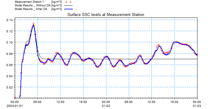
The results from the data assimilation model are shown in the below figure, showing the SSC levels at measurement station 1.

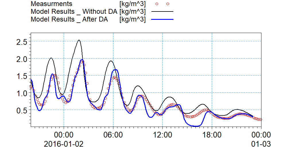Comparison between measured SSC levels and model results including data assimilation.

The figure below shows the errors introduced at the Northern Boundary by each of the ensemble members.

Error values introduced over the SSC levels at Northern Boundary Condition (Error Model 2).

Dredging in Harbor

In this example (download files) a section of a channel (with unidirectional current) including a harbor, where some dredging activities are going on, is modelled. The objective is to use data assimilation to improve the model predicting the SSC levels resulting from dispersion of spilled sediments from dredging activities. Two measurement points are assumed, one downstream inside the channel which shall be used for validation, and the other inside the harbor which shall be used for assimilation.

Model domain and bathymetry of the Harbor example, the two measurement points and the dredging point.

In order to simplify this exercise, the following assumptions are made:

• Data on SSC levels from two measurement stations is available, and it is assumed that they contain an error with standard deviation off 0.005 kg/m3.

Measured SSC levels at the two stations shown in the figure above.

• The current magnitude and directions at both open boundaries (East and West) are known.
• The initial conditions for SSC levels and seabed are thickness of 0.02 m and SSC = 0.001 kg/m3.
• The SSC boundary condition upstream is assumed zero and downstream is assumed zero gradient.
• The dredging rate is assumed constant 50 kg/s, however it is known that in practice it varies in time and can decrease to zero or increase up to 150 kg/s, which we hence model with a standard deviation of 100 kg/s.

The model results without data assimilation are not satisfactory when comparing to the measurements. The figure below shows the model results in comparison with measured SSC levels. The impact of considering a constant dredging rate is visible.

Comparison between measured SSC levels and model results without data assimilation.

The Data Assimilation module is added to the pfs setup file. The number of ensemble members is set to 10, and the Ensemble Kalmen Filter method (type 1) is chosen for assimilation.

[METHOD]
    type = 1
    algorithm = 2
    ensemble_size = 10
EndSect  // METHOD

The time step for beginning creating ensembles is set to 0, and the time step for applying data assimilation on the ensembles is set to 4 (after the start time step). The data assimilation time steps are set to equal to the main HD model time steps.

[TIME]
    start_time_step = 0
    start_time_step_assimilation = 4
    time_step_factor_assimilation = 1
EndSect  // TIME

One model error is introduced in the Data Assimilation section:

• Model Error on dredging rate magnitudes at the dredging source. Note that in this exercise the negative dredging rates are used as input, therefore in order to avoid positive “rate” values during simulation, a perturbation bound is introduced.

[MODEL_ERROR_1]
    type = 'MT_dredging'
    dredger_id = 1
    parameter_name = 'rate'

    [Error_Formulation]
        st_dev = 100
        perturbation_type = 'additive_bounded'
        propagation_type = 'AR(1)'
        propagation_parameter = 10800
        initialization_type = 1
        perturbation_bounds = -150, 0
    EndSect  // Error_Formulation
EndSect  // MODEL_ERROR_1

The measurement points are added to the measurement section with corresponding “include” type.

[MEASUREMENTS]
    number_of_independent_measurements = 2
    [MEASUREMENT_1]
        name = 'point1'
        include = 2
        measured_variable = 'MT%SSC_FRACTION_1'
        type = 1
        file_name = |..\obs\ssc_obs1.dfs0|
        item_number = 1
        position = 5334.211006192, 2611.515721263
        st_dev = 0.005
    EndSect  // MEASUREMENT_1

    [MEASUREMENT_2]
        name = 'point2'
        include = 1
        measured_variable = 'MT%SSC_FRACTION_1'
        type = 1
        file_name = |..\obs\ssc_obs2.dfs0|
        item_number = 1
        position = 3749.359434, 2149.496746
        st_dev = 0.005
    EndSect  // MEASUREMENT_2
EndSect  // MEASUREMENTS

The “ENSEMBLE_IO” Output section is activated to write out the error values. The type of files follows the nature of the Model Error. For example, the dredging source errors are written out as dfs0 files because they’ve been applied over the source value. The resulting errors on the “State Variable” (which in this case are the SSC values) will be written out as dfsu files. The “type” tells if it writes out the mean state (type=1), or all the ensemble members (type=2).

[ENSEMBLE_IO]     
    [INPUT]
        type = 0
    EndSect  // INPUT

    [OUTPUTS]
        number_of_outputs = 1
        [OUTPUT_1]
            type = 2
            file_name_area = 'State_Area.dfsu'
            file_name_volume = 'State_Volume.dfsu'
            file_name_err01_mtdredging = 'State_err01_dredging.dfs0'
        EndSect // OUTPUT_1
    EndSect  // OUTPUTS
EndSect  // ENSEMBLE_IO

The “Diagnostic Output” writes out the state variable (SSC variable) for all the ensemble members as well as their mean value. This can be done at the measurement points, or at any desirable point inside the domain.

[DIAGNOSTICS]
    [OUTPUTS]
        number_of_outputs = 3
        [OUTPUT_1]
            type = 1
            measurement_id = 1      
            file_name = 'diagnostics_meas1.dfs0'        
        EndSect  // OUTPUT_1

        [OUTPUT_2]
            type = 1
            measurement_id = 2      
            file_name = 'diagnostics_validation.dfs0'
        EndSect  // OUTPUT_2

        [OUTPUT_3]
            type = 2
            position = 5334.211006192, 2611.515721263
            variable_name = 'err01_mtdredging'
            file_name = 'diagnostics_err01_MT_dredging.dfs0'
        EndSect  // OUTPUT_3
    EndSect  // OUTPUTS
EndSect  // DIAGNOSTICS

The results from the data assimilation model are shown in the figures below, showing the SSC levels at measurement station 1 (DA) and 2 (validation).

Comparison between measured SSC levels and model with data assimilation at point of assimilation.

Comparison between measured SSC levels and model with data assimilation at validation point.

SW

Southern North Sea SW

Download files

Domain

The model area from the Hollandse Kust metocean project (Dutch Offshore Wind Farm Zone) was used for this example. The mesh was de-refined from 55000 (original set-up) to 2000 elements. Twenty-one stations for wind and wave observations are available in the area. Meanwhile, satellite altimetry provides wave and wind observations for the entire domain (lower accuracy of such data near the coast has to be considered).

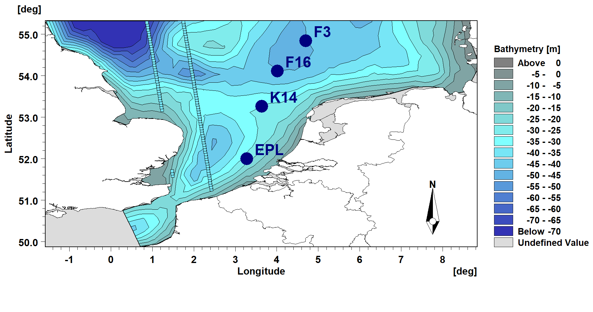
Area of interest with location of wave observations (buoys, tracks from Cryosat2).

Input

The setup is created for a storm that occurred late October 2017. Stations and track measurements are be given in .dfs0 format. The mesh (de-refined) of the domain is in .mesh format. The wind forcing is obtained from the global atmospheric model CFSR (here the default wind and not the bias corrected wind is used). The hydrodynamic conditions from the corresponding hydrodynamic Dutch model (which calls HD boundaries from the regional HD nemo model) and the boundary conditions from the regional North Sea wave model (SWNS) are applied.

Settings for the DA module

The example is divided into 3 cases: A, B and C.

Run A. This run is a simple SW run without assimilation.

Run B. This is a free run to create a realistic ensemble of realizations that are located around the observations (an ensemble of 10 members is used here). The wind is perturbed to create the ensemble. No assimilation is applied in this run.

Run C. This is the assimilation run using the EnKF method and 10 ensemble members. Three stations are assimilated (EPL, K14 and F3) and one station is used for validation (F3). The assimilation time step was set equal to the simulation time step, i.e. 600s in the example.

Run D. This is another assimilation run using the EnKF method and 10 ensemble members. In this case, only the significant wave height from altimetry in the domain is assimilated. The satellite data is retrieved from the RADS database (http://rads.tudelft.nl/rads/rads.shtml).

Settings for the model error:

[MODEL_ERROR_1]
    type = 'wind'
        [Error_Formulation] 
            st_dev = 1.5             
            propagation_type = 'AR(1)' 
            propagation_parameter = 10800
            initialization_type = 1 

            horizontal_discretization_type = 2 
            horizontal_grid_spacing = 80000  

            horizontal_corr_function = 1  
            horizontal_corr = 500000 
    EndSect
EndSect  // MODEL_ERROR_1

The u- and v- components of the wind is perturbed by adding 1.5m/s additive noise on a 80km grid with a spatial correlation length scale of 500km. This wind error is propagated in time by a AR(1) process with a half time of 3 hours (10800s).

Results

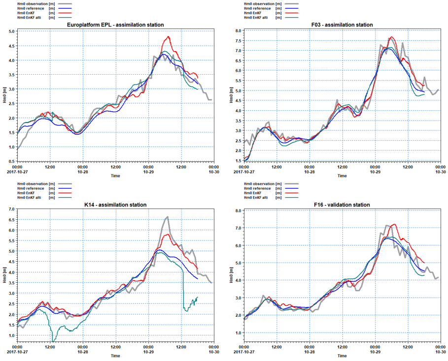
Comparisons of significant wave height (Hm0) at the assimilation stations EPL, K14 and F3, and at the validation station F16. Grey=observations, blue=reference SW run, red=assimilation run of 3 stations with EnKF (10members) and green=assimilation run of Cryosat2 tracks.

Please note that the number of stations that are assimilated has an impact on the results. The more the stations, the better the results. For this case, assimilation of altimetry tracks leads to improvements only if the initial set up and forcings have a poor quality.