Introduction to data assimilation

Data assimilation is the process of continuously improving a dynamical model by integrating observations. It is not an offline, post-processing method for error correcting results after completing the simulation. Rather, it's an integral part of the simulation process where the model is updated when an observation is received before proceeding with the next time step.

The purpose of this text is to give an intuitive and simple introduction to the theory behind the data assimilation methods used in MIKE FM. It prioritizes understanding over mathematical rigor.

The dynamical system

A dynamical system (such as a moving train or an ocean) can at a given time $t$ be characterized by its state $x$. A linear system may in discrete-time be described by the following linear matrix equation evolving the previous state at time ${k-1}$ to time $k$

$$x_k = F x_{k-1} + B u_k + \varepsilon_k$$

where $F$ is the prediction matrix, $u$ is an external forcing and $B$ is the control input matrix that relates the forcing to the state. Finally, $\varepsilon$ represents the process noise which we assume to be drawn from a zero-mean multivariate Gaussian distribution with covariance matrix $Q$. (The matrices $F, B$ and $Q$ do not need to be constant in time but the subscript k have been omitted for brevity).

Example

Train on a track

To easier understand the dynamical system, consider a moving train on a one-dimensional track. The state is here represented by the train's position and velocity (state size is n=2) and the "train system" can be expressed by the above linear matrix equation. Think of the control as effect of change in the throttle or breaking.

Observations

Measurements (which we typically call "observations") can be performed on the system using the following expression

$$y_k = H x_k + \delta_k$$

where $H$ is the observation operator (that maps the state space into the observation space) and $\delta$ is the observation noise assumed to have zero-mean and be normal distributed with covariance matrix $R$.

For a simple scalar measurement $y_k$ (e.g. water level in a point), the observation operator $H$ may simply be the matrix that "selects" the right variable (water level) in nearest point in the state vector $x_k$.

State estimation

Unfortunately, we cannot directly observe the true state of the system $x_k$. But we can estimate it and we denote our best estimate by $\hat{x}_k$ and it's associated covariance $P_k$. The covariance matrix $P_k$ represents the uncertainty associated with our best estimate $\hat{x}_k$ - the diagonal elements gives the variance of each element of $x_k$ whereas the off-diagonal elements tells us the about the correlation.

Note

For a scalar system, we typically denote our best estimate (the mean) by $\mu$ and the variance $\sigma^2$.

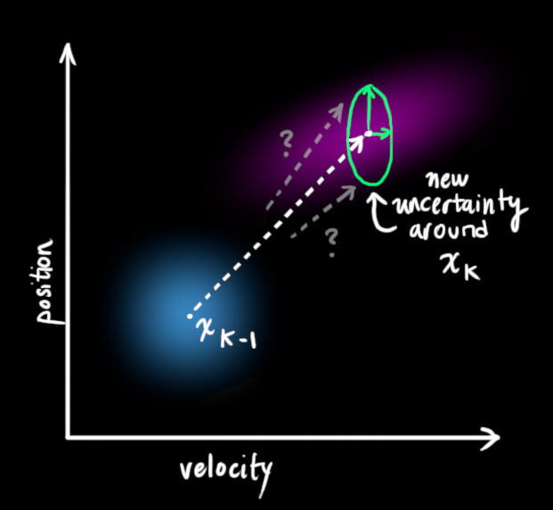
Assuming that our system has the above dynamic description we can estimate the new state using the model

$$\hat{x}_k = F \hat{x}_{k-1} + B u_k \;$$

$$P_k = F P_{k-1} F^T + Q$$

In other words, the new best estimate of the state $\hat{x}_k$ is a prediction $F \hat{x}_{k-1}$ made from previous best estimate $\hat{x}_{k-1}$, plus a correction for known external influences $B u_k$.

The new uncertainty $P_k$ is predicted from the old uncertainty $P_{k-1}$ plus the influence from additional uncertainty from the environment $Q$ (process noise). The expression for $P_k$ can be derived by evaluating the expected value of the state "error" i.e. the difference between $x_k$ and $\hat{x}_k$. We therefore often denote $P_k$ the state error covariance matrix.

The next step is to improve our (uncertain) estimate of the state by using (uncertain) information observation of our system. The observation model reads

$$\hat{y}_k = H \hat{x}_k$$

Luckily, there is a "best" way to combine an uncertain state estimate $\hat{x}_k$ with gaussian errors and uncertain observation with gaussian errors - that is called BLUE and is the central part of the Kalman filter.

Notation

Symbol	Description
n	Length of the state vector, state size
p	Number of observations
$x$	State vector, size n
$u$	Forcing vector
$F$	Prediction/Forecast matrix
$Q$	Process noise covariance matrix, size n-by-n
$P$	State error covariance matrix, size n-by-n
$y$	Observation vector, size p
$H$	Observation matrix, size p-by-n
$R$	Measurement error covariance matrix, size p-by-p

Combining two Gaussians

Consider a Gaussian $G$ with mean $\mu$ and variance $\sigma^2$

$$G(x,\mu, \sigma) = \frac{1}{\sigma \sqrt{2\pi}} e^{-\frac{(x-\mu)^2}{2\sigma^2}}$$

We claim that the product of two Gaussians is a new Gaussian with mean $\tilde{\mu}$ and variance $\tilde{\sigma}^2$

$$G(x, \tilde{\mu}, \tilde{\sigma}) = G(x,\mu_1, \sigma_1) G(x,\mu_2, \sigma_2)$$

By substituting the definition into this expression and using algebraic manipulations it can be shown that the product is indeed a Gaussian with mean and variance

$$\tilde{\mu} = \mu_1 + \frac{{\sigma_1}^2 (\mu_2 - \mu_1)}{{\sigma_1}^2 + {\sigma_2}^2}$$

$$\tilde{\sigma}^2 = \sigma_1^2 - \frac{{\sigma_1}^4}{{\sigma_1}^2 + {\sigma_2}^2} \qquad$$

We can simplify these expressions by factoring out a part which we call $k$

$$\tilde{\mu} = \mu_1 + k (\mu_2 - \mu_1)$$

$$\tilde{\sigma}^2 = \sigma_1^2 - k \sigma_1^2 \qquad \quad$$

where $k$ is

$$k = \frac{{\sigma_1}^2}{{\sigma_1}^2 + {\sigma_2}^2}$$

Notice that the new variance is smaller than the original variance and that the "gain" $k$ is simply a weighting between the two variances.

The above product is Bayes Theorem applied to univariate Gaussian distributions. The first distribution $G(x,\mu_1, \sigma_1)$ is the prior (the first estimate) and the second $G(x,\mu_2, \sigma_2)$ the likelihood (the observation/evidence). The product distribution $G(x, \tilde{\mu}, \tilde{\sigma})$ is the posterior (the updated estimate).

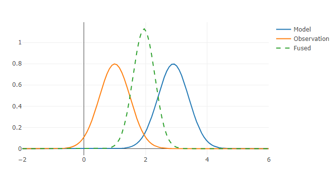
The result of two gaussian distributions with equal variance.

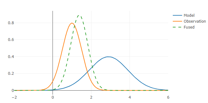
The result of two gaussian distributions with different variances.

Try yourself.

The Kalman filter (KF)

The Kalman filter is a simple yet powerful way of combining information in the presence of uncertainty. It was invented more than 50 years ago by Rudolf E Kálmán. It helped the Apollo mission reach the moon and is today part of every satellite navigation device including every smartphone. It utilizes the above shown fact that the product of two Gaussian distributions is also a Gaussian distribution.

The Kalman filter algorithm consists of two stages: forecast and analysis (also called prediction and update) - indicated by a superscript $f$ or $a$ below (the $\hat{\cdot}$ is omitted to simplify the exposition). The forecast stage advances the model and the model error covariance one time step:

Forecast: $$ x^f_k = F x^a_{k-1} + B u_k \; $$

$$P^f_k = F P^a_{k-1} F^T + Q$$

In the presence of observations $y_k$, the analysis (or update) stage corrects this estimate by

Analysis: $$ x^a_k = x^f_k + K (y_k - H x^f_k) $$

$$P^a_k = P^f_k - K H P^f_k \qquad$$

Where the Kalman gain matrix is given by

$$K = P^f H^T (H P^f H^T + R)^{-1}$$

The analysis equations is simply the multi-dimensional equivalent of the above shown combination of Gaussian distributions. The observation operator complicates the expression, but is simply a mapping from state space onto measurement space. If all state vector elements are observed (e.g. if both position and velocity are measured in the train example above) then $H$ can be removed from the equations and it's easier to see that the update is simply the multi-dimensional equivalent to the above product of Gaussian distributions.

The difference ($y - H x$) between the observation $y$ and the model forecast mapped to the same element $H x$ is called the innovation. The update is a linear combination of the model forecast (the prior) and the observation (the likelihood).

The update minimizes the variance under the assumption that the model is linear, all errors are Gaussian with zero mean and the model and measurement errors are uncorrelated. It is therefore called the Best Linear Unbiased Estimator (BLUE).

Large geophysical dynamical systems

A large non-linear geophysical system (such as a part of the ocean) may be expressed by the following equation:

$$x_k = \Phi (x_{k-1}, u_k, \theta_k, \varepsilon_k)$$

where $\Phi$ is a non-linear forecast operator advancing the system from the previous state $x_{k-1}$ to the new state $x_{k}$ under the influence of external forcings $u_k$, system parameters $\theta_k$ and process noise $\varepsilon_k$. In MIKE FM, $\Phi$ would be integrating the system one time step forward. The state vector could for MIKE FM be the collection of the discretized prognostic variables (e.g. water level, u- and v-current components in all elements) - essentially the information needed for a hotstart.

For small linear models the error covariance can be directly calculated from the model operator. But for large geophysical models such as the MIKE FM models where the state size $n$ is often very large ($n > 10^5$) and the model is non-linear it is not possible to explicitly construct the error covariance matrix and hence not possible to apply the Kalman filter.

All hope is however not lost, as we can still use the above forecast-analysis stages and the BLUE to update our model when we have observations. The main challenge is how to estimate the model error covariance $P$ as this is the key component of the Kalman gain matrix. $P$ gives us the information about the covariance (correlations) across space and across different variables (e.g. how change in water level in one point co-varies with change in u-component of the current in another point 2km away).

The MIKE FM data assimilation module provides two ways of describing the model error covariance $P$:

Optimal interpolation (OI) which uses a simple prescribed static and uni-variate description of $P$.

Ensemble Kalman filter (EnKF) which uses an ensemble of model realizations to estimate $P$ by the sample error covariance $\tilde{P}$.

Optimal interpolation (OI)

Optimal interpolation is a commonly used and relatively simple form of data assimilation. The term "optimal" is misleading because the method is only optimal if we know the involved error covariances which we in practice never do. It is therefore far from optimal and for this reason it is sometimes also referred to as statistical interpolation.

The model error covariance $P^f$, which is often called the background error covariance $P^b$ in the OI literature, is given analytically by a simple distance function (often a Gaussian) estimating the error covariance between two points. This description is uni-variate (e.g. it does not tell us how water level in one point co-varies with u-current component in another point) and often isotropic and can for geometrically complex domains lead to false correlations (e.g. across land masses). But it's simple and fast and can sometimes give good results.

The implemented OI algorithm consists of the same two stages as the KF algorithm:

Forecast: $$ x^f_k = \Phi_{FM} (x^a_{k-1}, u_k, \theta_k), $$

where $\Phi_{FM}$ is MIKE FM model forecast operator.

Analysis: $$ x^a_k = x^f_k + K (y_k - H x^f_k) $$

$$K = P^b H^T (H P^b H^T + R)^{-1}$$

where the state error covariance is static and shown with superscript $b$ for background. The algorithm has no forecast and analysis equations for the state error covariance as it is assumed constant.

The optimal interpolation implementation in MIKE FM allows the user to specify several sets of specifications each valid for one variable (e.g. water level) with its own model error covariance parameters: model standard deviation $\sigma$ and correlation length $L$ (both can be spatially varying) referring to specific measurements. See Optimal Interpolation and PFS Section Optimal Interpolation in the reference manual for more details.

The Ensemble Kalman filter (EnKF)

The Ensemble Kalman Filter (EnKF) (Evensen, 2003) is a popular Monte Carlo approximation of the KF, which uses an ensemble $x_1, x_2, \ldots , x_m$ of model realizations to approximate the state error covariance $P$. The different realizations (or members) are typically generated by randomly varying initial conditions, forcings or model parameters. Read MIKE FM Ensemble modelling to understand how an ensemble can be created. The ensemble should be constructed such that its spreading corresponds to the model error of the system.

By subtracting the mean state $\bar{x}$ from the ensemble matrix $E$ containing the state vectors of all ensemble $m$ members $E = [x_1, x_2, \ldots , x_m]$, we can construct the anomaly matrix $A = E - \bar{x}$. The state error covariance is now given by the following expression

$$ P = \frac{1}{m-1} A A^T $$.

Conversely, we can say that this factorization allows for a representation of the model state error covariance $P$ by the ensemble anomalies $A$. Representing $P$ via the ensemble anomalies makes it possible to use the Kalman filter update for large-scale geophysical systems like a MIKE FM model.

Notation

Symbol	Description
m	Number of ensemble members (ensemble size)
$E$	Ensemble (m members with state size n)
$\bar{x}$	Ensemble mean
$A$	Anomalies, $A = E - \bar{x}$

The EnKF algorithm

The forecast stage of the EnKF consists of propagation of each model realization potentially subject to different previous state, different forcings and different parameters:

Forecast: $$ x^f_{j,k} = \Phi_{FM} (x^a_{j,k-1}, u_{j,k}, \theta_{j,k}), \qquad \text{for} \; j = 1, ..., m$$

$$P^f_k = \frac{1}{m-1} A^f_k (A^f_k)^T$$

Note how the forecast error covariance $P^f_k$ is simply derived from the forecasted ensemble. It is not constructed explicitly in practice.

Analysis: In the presence of observations $y_k$, the analysis stage takes the following form updating the ensemble mean $\bar{x}$ and anomalies $A$ individually:

$$\bar{x}^a_{k} = \bar{x}^f_{k} + K (y_k - H \bar{x}^f_{k})$$

$$A^a_k = A^f_k T_R$$

where $K$ is the well-known Kalman matrix $$ K = P^f H^T (H P^f H^T + R)^{-1} \qquad \qquad $$

and $T_R$ is the ensemble transformation matrix which is constructed such that:

$$T_R: \qquad P^a = P^f - K H P^f, \quad A^a 1 = 0$$

We never construct the full $P$ or $K$. Either, $P$ and $K$ are constructed in only a few fixed points, or we use an algorithmic reformulation that avoids the need for explicit construction of these matrices.

All EnKF implementation in MIKE FM are “deterministic” so-called square-root type filters (ESRF) opposed to the original stochastic perturbed-measurements-EnKF proposed by Evensen 1994. ESRF performs much better than perturbed-measurements-EnKF for small ensembles (e.g. m<100). Three different ESRF schemes or algorithms can be chosen: one with serial processing of measurements and two using the ensemble transform Kalman filter formulation.

Different algorithms

Serial ESRF The serial ESRF (algorithm 1) also called the Potter scheme processes one independent measurement at a time and only works for station data (e.g. water levels from tide gauge stations). It explicitly constructs the error covariance $P$ and Kalman gain matrix $K$ but only at the few points where it is needed (where measurements are available).

The serial ESRF allows for the use of error covariance smoothing and for the possibility of saving the error covariance in the measurement points (see ErrCovIO) for further analysis or for a "steady" run.

Ensemble transform Kalman filters
The Ensemble Transform Kalman filter (algorithm 3) and the related Deterministic Ensemble Kalman Filter (algorithm 2) avoid explicit construction of the error covariance $P$ or Kalman gain matrix $K$ which has several advantages from a computational point of view and it allows for general measurements that may change size and position over time (e.g. satellite tracks). The Deterministic Ensemble Kalman Filter is an approximation to the Ensemble Transform Kalman filter, which is computational faster and more stable in extreme situations. The drawback of these schemes is that they do not permit the user to save the error covariance output (e.g. for a steady run) and that the smoothing is less effective (see Random anomaly tail smoothing).

Inflation techniques

The Ensemble Kalman Filter uses the sample error covariance in place for the real error covariance which unavoidably leads to a sampling error and an underestimation of the variance. When applying the EnKF, assimilation will often reduce the ensemble spread too much. Inflation techniques are ad-hoc compensation strategies to minimize this effect. The following techniques are available in MIKE FM:

• Rfactor_anomalies (preferred)
• spread_reduction_factor

Use only one of these at a time! Read pfs section METHOD for more specification details.

Regularization of the EnKF

The EnKF approximates the “true” error covariance by the sample error covariance through the ensemble representation. The limited size of the ensemble inevitably introduces noise which increases with decreasing ensemble size. The noise is evident both in spatial and temporal directions.

In practice, we wish to use the Ensemble Kalman Filter with as few ensemble members as possible to minimize the computational cost associated with ensemble simulations. To get useful results from small ensembles, we often need apply regularization to minimize the noise. Localization is a regularization technique to minimize the noise in the spatial direction. Error covariance smoothing is a regularization technique to minimize the noise in the temporal direction.

Localization

The spatial noise in the error covariance often referred to as spurious long-range correlations may be accounted for by so-called localization, where the effect of the update is decreased gradually away from the point of observation by multiplying by a taper function. In the Serial ESRF, this can be conveniently done directly on the error covariance P (called covariance localization CL). In the ETKF and DEnKF, the so-called Local Analysis (LA) performs the localization by element-by-element formulation of the update equations. From a user perspective, however, there is no difference as the localization is specified in the same way.

Temporal smoothing in the serial ESRF

If observations are scalar and fixed in space (like tide gauge stations), the Serial ESRF gives us the opportunity to reduce the noise in the temporal direction by smoothing the error covariance exponentially with a smoothing factor s with

$$P_{sm}^k = s P^k + (1-s) P_{sm}^{(k-1)}, \qquad \qquad s \in [0;1]$$

which is a good approximation for slowly-varying error covariance. In practice for tidal and storm surge models, smoothing of the error covariance allows for the use of much smaller ensemble e.g. 8 instead of 50. The choice of smoothing factor becomes a tuning parameter and a compromise between a reduction of high-frequency error covariance noise and maintaining the EnKF’s ability to adapt dynamically to new situations. The smoothing factor s is determined from desired half-life $\tau$ and the time step length $\Delta t$ by the relation

$$s = 1 - 0.5^{\frac{\Delta t}{\tau} }$$

In practical coastal-ocean applications, a smoothing factor corresponding to a 3-hour half-life has shown to be a good choice. If the time step $\Delta t$ is 5 minutes, then the smoothing factor amounts to s = 0.0191.

The figure below shows time series of a single element in three different approximations of the error covariance matrix $P$. Notice how noisy the 8 member $P_m$ appears and how much better the smoothed 8 members $P_{smooth}$ becomes. Smoothing inevitably introduces a time lag as it uses information from previous time steps, which the figure also reveals.

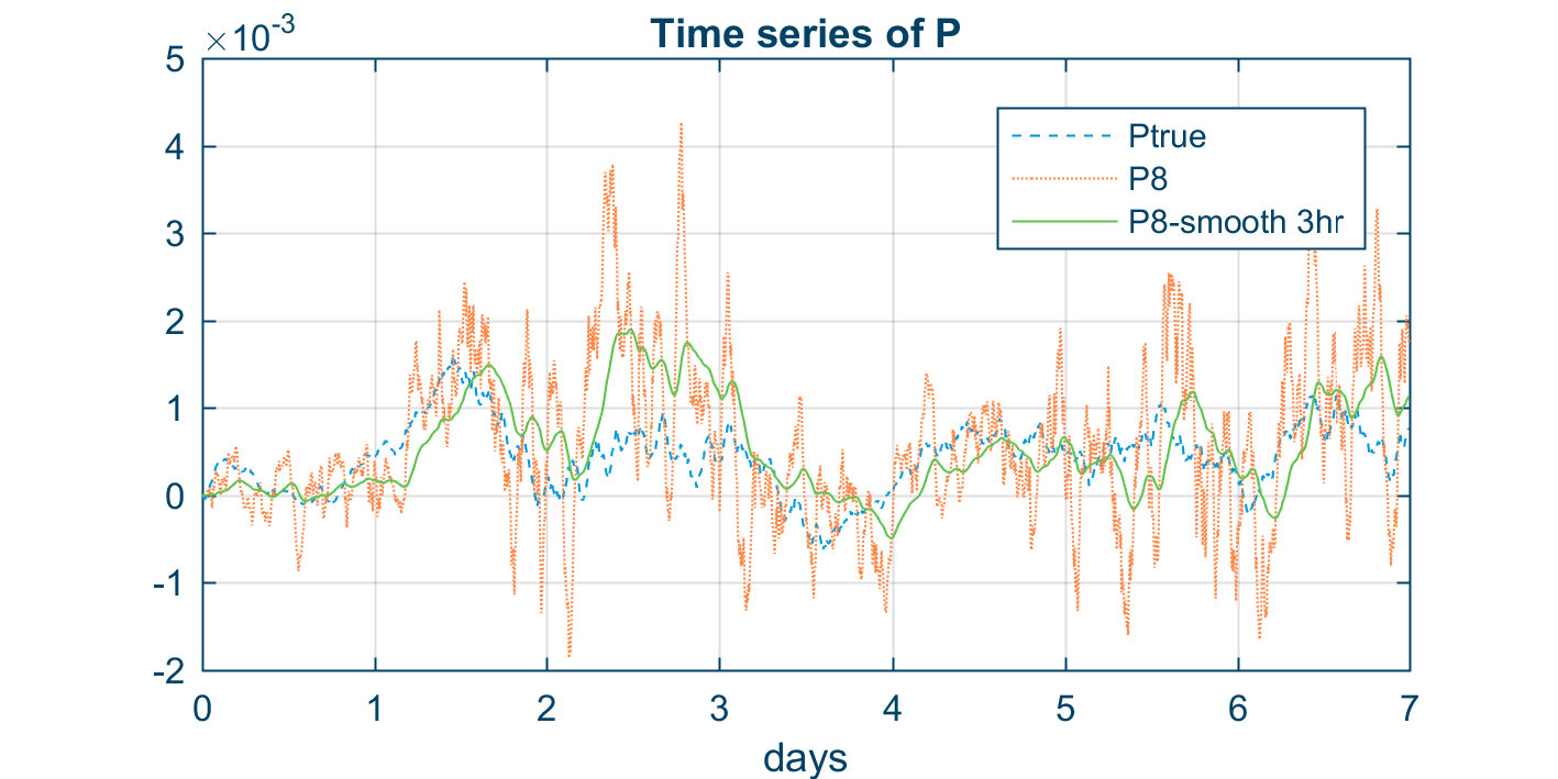
Time series of three different error covariances: the converged $P_{true}$, a noisy 8 member $P_m$ and a 3-hour smoothed $P_{smooth}$ also with 8 members.

Temporal smoothing in the Ensemble Transform filters

(see Random anomaly tail smoothing).