Reference manual for MIKE FM Data assimilation¶

This page contains possible settings allowed by the DA module.

PFS file¶

To make the engine recognize that your model is a DA model, it needs to be told to look for the DA section in the PFS by adding the following to the [MODULE_SELECTION]:

   [MODULE_SELECTION]     
      mode_of_data_assimilation_module = 2
   EndSect  // MODULE_SELECTION

This will make the engine look for the PFS section [DATA_ASSIMILATION_MODULE].

PFS section `[DATA_ASSIMILATION_MODULE]`¶

Below sections of this user guide correspond to different PFS sections in the overall DA PFS structure

[DATA_ASSIMILATION_MODULE]
    [TIME]
    [METHOD]
    [ENSEMBLE_FORCINGS]
    [MODEL_ERROR_MODEL]
    [MODEL_STATE_SPACE]
    [MEASUREMENTS]
    [ESTIMATOR]
    [ERRCOV_IO]
    [ENSEMBLE_IO]
    [DIAGNOSTICS]
EndSect

Time¶

The TIME section controls the time stepping of the DA module. The settings are relative to the overall time stepping of the MIKE FM model.

The TIME section offers control over the two levels of time stepping in the DA module:

DA module time stepping - effectively only when the DA module should start (the step factor will always be 1)
Assimilation times - concerning only assimilation

A few things should be noted here:

Error propagation: always happens before model propagation and will be done on DA module time steps
Model propagation: after error propagation and at all time steps
Diagnostics: diagnostics outputs and statistics will be done at all steps (step_factor=1) within DA module start-end after propagation
Assimilation: will be done at assimilation steps after propagation (cannot be less than 1)
Ensemble outputs: will be done within DA module start-end, but can have different step-factor and other start and end

PFS Section `TIME`¶

[TIME]
    start_time_step = 0

    start_time_step_assimilation = 1200
    time_step_factor_assimilation = 30  
EndSect

Keyword	Description	Values
start_time_step	start step of DA module relative to the overall time stepping	default:0
start_time_step_assimilation	starting point of assimilation relative to the overall time stepping (would often be larger than 1 to allow the ensemble to spread first before assimilating)	default: start_time_step+1
time_step_factor_assimilation	step factor of assimilation relative to the overall time stepping (must be an integer multiple of the module time_step_factor)	default: time_step_factor

Method¶

The METHOD section lets you set the overall properties of your data assimilation model.

DA Type	Propagation	Assimilation	Errcov
0:Free run	Ensemble	No	N/A
1:EnKF, with algorithms 1. Serial ESRF 2. DEnKF 3. ETKF	Ensemble	Yes	Dynamic
2:Optimal Interpolation	1	Yes	Static
3:Steady	1	Yes	Static
4:EnOI	1	Yes	Static

Ensemble model and free run¶

Type 0. We create an ensemble of slightly different realizations of our model by either perturbing initial conditions, forcings, model parameters or any combination hereof. The next chapter details how this is done in MIKE FM. For now, it is enough to realize that an ensemble model consist of m realizations---called members---of our system state. Each of these are propagated individually one time step forward at a time by the numerical model e.g. MIKE 3 FM HD. On top of this, the DA model also has a separate mean state, which is not propagated by the numerical model. We use the term “free” or “open loop” run for an ensemble model run without assimilating measurements (type 0).

It is advised to perform a “free” run and assessing the ensemble spread etc before proceeding with a data assimilation model. The ensemble should have enough spread to “cover” the observations in some sense.

The output of a free run may also be used for defining a static background ensemble which can be used as input to an Ensemble OI model (see EnsembleIO below).

The free run may be conducted with just one ensemble member and without perturbation (no model errors). The model run will then be the same as the base model (e.g. MIKE 21 HD or MIKE 21 SW) but with the validation and output capabilities of the DA engine. It can be useful as a baseline run as the very first simulation.

Ensemble Kalman filter¶

Type 1. Now having an ensemble of states and thereby the anomalies, we can estimate the model error covariance P for any variable and in any point of our domain. This sample error covariance is perhaps the most important component in the ensemble Kalman filter EnKF. In practice two steps needs to be performed:

Forecast: Propagate all ensemble members (and model errors --- see Model Errors).
Update: assimilate observations using the update equation. Mean state and anomalies are updated separately. Each update is a linear combination of anomalies which ensures physically sound updates.

The forecast step is performed for every numerical model time step, the update step is performed after some forecast steps (e.g. when measurements are available).

All EnKF implementation in MIKE FM are “deterministic” so-called square-root type filters (ESRF) opposed to the original stochastic perturbed-measurements-EnKF proposed by Evensen 1994. ESRF performs much better than perturbed-measurements-EnKF for small ensembles. Three different ESRF schemes or algorithms can be chosen: one with serial processing of measurements and two formulated in the ensemble transform Kalman filter formulation.

A serial algorithm (algorithm 1) The serial ESRF also called the Potter scheme processes one independent measurement at a time and only works for 0D station data (e.g. water levels from tide gauge stations). It allows for the use of error covariance smoothing (see Regularization) and for the possibility of saving the error covariance in the measurement points (see ErrCovIO) for further analysis or for a “steady” run (see Steady ).

Ensemble transform Kalman filters (algorithm 2 and 3) Ensemble Transform Kalman filters and the related Deterministic Ensemble Kalman Filter avoid explicit construction of the error covariance or Kalman gain matrix which has several advantages from a computational point of view and it allows for general measurements that may change size and position over time (e.g. satellite tracks). The drawback of these schemes is that they do not allow for the possibility to save error covariance output (e.g. for a steady run) and that the smoothing is less effective (see Regularization).

Steady¶

Type 3. If a previous EnKF (type 1) run have been made with the serial algorithm (algorithm 1) and the average error covariance outputs have been saved, then a so-called “Steady” run can be performed by setting the type to 3 and inputting the previously saved time-averaged error covariance files (see ErrCovIO). In this case the model error covariance will be static (in contrast to the dynamic nature of the EnKF) but multivariate and anisotropic and only require one member. It will therefore be almost as fast as the base MIKE FM model. The results are in most cases less accurate than the full EnKF but much cheaper and typically significantly better than using simpler OI techniques.

Ensemble optimal interpolation¶

Type 4. EnOI is similar to Steady since it requires integration of only one member and is hence computational cheap. It is more general, however, as it is not limited to using a fixed number of station measurements. EnOI works by loading a number (e.g. 100) of background anomaly vector from a previously run ensemble model and using these to perform the update using measurements of any size and in any part of the domain (with algorithm 1 or 2).

The procedure is to first run an ensemble model for a shorter period with high temporal resolution of the ensemble output (see EnsembleIO) and then run a post-processing tool that calculates anomalies from each time step and randomly selects a number (e.g. 100) anomalies (from different members and different time steps). Then EnOI model (type 4) is created reading the anomaly files using the ensemble input (see EnsembleIO).

In EnOI, the strength of the assimilation needs to be calibrated by setting Rfactor_all – typically to a relatively low number e.g. 0.05.

Optimal Interpolation¶

Type 2. Optimal Interpolation (OI or "statistical interpolation") is a relatively simple univariate data assimilation technique assuming that the model error covariance is static. In most OI implementations including this, the so-called background error covariance describing the model error statistics is assumed to be isotropic and univariate. The implementation in MIKE FM does however allows for a spatially varying error covariance description if the user supplies a map of model standard deviation and horizontal correlation length scale. This gives the user the ability to describe long range correlations in offshore areas and short range correlations in coastal waters or to disregard some areas during the model update.

In OI a single variable (the observed) is updated directly at the point of observation and decreasing gradually away from the point of observation at a scale specified by the user. The "gain" at the observation point is a weighted estimate between the model variance P (supplied by the user as "st_dev") and the measurement variance R (supplied by the user in the MEASUREMENT section below): gain=P/(P+R).

$x_a = x_f + K (y - H x_f)$

where the gain matrix $K$ giving the "optimal" solution (minimum variance) is given by

$K = P H^T (H P H^T + R)^{-1}$

But note that this solution is only "optimal" if the error covariance $P$ is really known.

Note

Only the observed variable will be updated! This can lead to model imbalance (e.g. if you update water level in a HD model without changing velocities, salinity and temperature). The update assumes a simple distance-based model error covariance structure (isotropic, univariate) which is unrealistic.

Note

The current implementation of Optimal Interpolation has been added after release of MIKE Zero 2020. Previously, type 2 assimilation referred to a similar section called SIMPLE.

Local approach¶

The above OI approach is global in the way that updates all elements at the same time and principally using all measurements (although the effect of the update will linger off away from the measurement with the specified horizontal correlation length scale). If you have many measurement points (e.g. a satellite map) this can be too heavy for the model. A local_approach exists as an alternative to the above "global approach". The local approach updates one model element at a time but only considering a small number of nearest measurement points.

Inflation and R-factor¶

The ensemble Kalman filter uses the sample error covariance in place for the real error covariance (which is infeasible for large systems) this unavoidably leads to a sampling error and an underestimation of the variance. When applying the EnKF in practice, assimilation will often reduce the ensemble spread too much. R-factor-anomalies and spread_reduction_factor are two ad-hoc compensation strategies to minimize this effect.

An Rfactor_anomalies larger than 1.0 works by increasing the uncertainty of the measurement (which is described by the measurement error covariance matrix R) when updating the anomalies relative to when updating the ensemble mean. This gives a larger spreading in the ensemble.

Alternatively, spread_reduction_factor allows you to directly modify the spread reduction which the ensemble experience upon assimilation. The spread reduction will typically be too strong due to the small ensemble size and a spread_reduction_factor smaller than 1 will then limit this effect.

PFS Section `METHOD`¶

[METHOD]
    type = 1               // 0=Free, 1=EnKF (ensemble), 2=OI, 3=Steady, 4=EnOI 
    ensemble_size = 10
    algorithm = 1          // (for type=1) 1=serialESRF, 2=DEnKF, 3=ETKF       

    spread_reduction_factor = 1.0
    Rfactor_anomalies = 1.0 // inflation only where model was updated (e.g. 2.0)        
    Rfactor_all = 1.0      // factor on st_dev for *all* measurements     
EndSect  // METHOD

Keyword	Description	Values
[METHOD]	Section for overall DA settings
type	Type of data assimilation	0: No assim. (“free” run) 1: Ensemble Kalman filter 2: OI 3: Steady 4: Ensemble OI Default value: 1
ensemble_size	Number of ensemble members if type=0, 1 or 4. Note that in case of type 4 the ensemble is static!	Default value: 10
algorithm	Algorithm or scheme to use in EnKF (type=1)	1: Serial ESRF 2: DEnKF 3: ETKF Default value: 1
spread_reduction_factor	Factor to modify the spread reduction which occurs during assimilation	Typical value is 0.5 Default value: 1.0 (off)
Rfactor_anomalies	Alternative to inflation where a factor is multiplied on the measurement error covariance R only when updating anomalies. Don't use both Rfactor_anomalies and spread_reduction_factor.	Typical value is 2.0 Default value: 1.0 (off)
Rfactor_all	A quick way to adjust error level on all measurements by a factor. Used in EnOI (type=4) to adjust effect of assimilation.	In case of EnOI it will typically be relatively small e.g. 0.05. Default value: 1.0 (off)

PFS Section `OPTIMAL INTERPOLATION`¶

If type 2 assimilation is selected, the subsection OPTIMAL_INTERPOLATION needs to be specified. The method is univariate but can be applied for several variables after each other

[METHOD]
    type = 2       // 0=Free, 1=EnKF (ensemble), 2=OI, 3=Steady, 4=EnOI 
    [OPTIMAL_INTERPOLATION]
        number_of_variables = 2
        [VARIABLE_1]  
            // add specification here
        EndSect 
        [VARIABLE_2]
            // add specification here
        EndSect 
    EndSect
EndSect

Optimal interpolation for a single variable can be specified either by:

a) specifying constant model error covariance characteristics (format=0):

    [VARIABLE_1]
        variable_name = 'surface elevation'
        horizontal_corr_function = 1
        format = 0
        constant_st_dev = 0.2
        constant_horizontal_corr = 50000    
    EndSect

or b) by supplying a file with spatially varying model error covariance characteristics (format=2):

    [VARIABLE_1]
        variable_name = 'surface elevation'
        horizontal_corr_function = 1
        format = 2
        file_name = |.\data\wl_background_error_covariance.dfsu|        
        item_number_st_dev = 1
        item_number_horizontal_corr = 2 
    EndSect

Keyword	Description	Values
[OPTIMAL_INTERPOLATION]	Section for specifying Optimal Interpolation DA
number_of_variables	Number of variables for which OI should be applied	Default value: 1
[VARIABLE_x]	Section for specifying OI for a variable Note! the variable needs to match the variable referenced in associated measurements
variable_name	Name of this variable (must be in state)	Default value: ''
algorithm	Algorithm for constructing and inverting the denominator of $K = P H^T (H P H^T + R)^{-1}$ .	1: Direct inversion 2: SVD inversion 3: Diagonal only Default value: 1
local_approach	Use the local element-wise approach where only a few local measurement points are used?	True/False Default value: False
number_of_local_points	if local_approach: how many nearest measurement points should be used for the update?	Default value: 5
horizontal_corr_function	Correlation function (e.g. Gaussian) to be used for distance weighting	1: Gaussian 2: Exponential 3: Gaspari & Cohn 4: Cubic exponential 5: Cubic polynomial 6: Step Default value: 1
vertical_corr_function	For 3d variables. Vertical version of horizontal_corr_function	Default value: horizontal_corr_function
format	Constant in space and time (0), Varying in space, constant in time (2) or varying in space and time (3).	Default value: 0
file_name	If format>=2: File name	Default value:
item_number_st_dev	Item num of model st_dev	Default value: 1
item_number_horizontal_corr	Item num of correlation length scale provided from file. If 0, then constant value will be read instead	Default value: 0
item_number_vertical_corr	For 3d variables: Vertical correlation. see item_number_horizontal_corr	Default value: 0
constant_st_dev	If format=0: The model uncertainty (to be weighted against the measurement uncertainty). Most be positive.	Default value: 0.0
constant_horizontal_corr	Constant correlation length scale if not provided from file	Default value: 100000.0
constant_vertical_corr	For 3d variables: Constant vertical correlation length scale.	Default value: 1000.0

ENSEMBLE_FORCINGS¶

If an ensemble forcing is available (e.g. ensemble wind from GFS or ECMWF) it can be used to force your ensemble FM model by using the ENSEMBLE_FORCINGS section. The ensemble members of the forcing needs to be in the same dfs file as different items. If the forcing requires several items, e.g. speed and direction for wind forcings in SW, all most be given as ensemble forcing items.

ENSEMBLE_FORCINGS is new in release 2022 update 1.

Ensemble item numbers imputation¶

Usually, ensemble input files are structured such that the number and sequence of variable items (e.g. pressure, x-velocity, y-velocity) are the same for all ensemble members. The engine can use this structure to impute (guess) the ensemble item numbers if they are not all given. It is enough for the user to provide ensemble_item_numbers = 1, 4 for the engine to guess 1, 4, 7, 10, 13 (for 5 members).

Available ensemble forcings per model¶

Hydrodynamic module HD

forcing_type	Specification
wind	format=1 (constant in space): 2 items: * `item_name`='speed' * `item_name`='direction' format=3 (variable in space): 3 items: * `item_name`='pressure' * `item_name`='x_velocity' * `item_name`='y_velocity'

Spectral wave module SW

forcing_type	Specification
wind	Wind type=1 (speed/direction): 2 items: * `item_name`='speed' * `item_name`='direction' Wind type=2 (wind components): 2 items: * `item_name`='x_velocity' * `item_name`='y_velocity'

PFS Section `ENSEMBLE_FORCINGS`¶

If the model is an ensemble SW model the following section can be used to specify how it shall read the ensemble forcing.

[ENSEMBLE_FORCINGS]
    number_of_forcings = 1
    [FORCING_1] 
        forcing_type = 'wind'
        number_of_items = 2

        [ITEM_1]
            item_name = 'speed'
            ensemble_item_numbers = 1, 3, 5
        EndSect 

        [ITEM_2]
            item_name = 'direction'
            ensemble_item_numbers = 2, 4, 6
        EndSect 
    EndSect 
EndSect

Keyword	Description	Values
[ENSEMBLE_FORCINGS]	Section for specifying ensemble forcings
number_of_forcings	Number of ensemble forcings	Default value: 0
[FORCING_x]	Section for specifying a single forcing
forcing_type	Name of this forcing (e.g. wind)	Default value: ''
number_of_items	Number of items for this forcing	Default value: 1
[ITEM_x]	Section for specifying a single item
item_name	Name of this item (depending on the forcing), e.g. "speed"	Default value: ''
ensemble_item_numbers	Item numbers for each ensemble member, e.g. 1, 4, 7. Note: duplicate entries are not allowed.	Default value:

Model errors¶

The ensemble of model states in a MIKE FM DA model is created by stochastically perturbing model forcings, initial conditions or model parameters. These perturbations are called model errors. This section focuses on specifying the MODEL_ERROR_MODEL pfs section, if you need to understand how ensemble modelling works in MIKE FM then read the page on ensemble modelling in MIKE FM.

PFS format¶

The PFS section for specification of the model errors has its own section. It has the following overall format:

[MODEL_ERROR_MODEL] 
    Number_of_model_errors = 2
    [MODEL_ERROR_1] // (…)
    [MODEL_ERROR_2] // (…)
EndSect

The child sections to ´MODEL_ERROR_MODEL´ are individual errors, e.g. MODEL_ERROR_1. Note that any error type can have more than one model error, e.g., one representing “slow” dynamics and another representing “fast” dynamics.

List of model errors per FM module¶

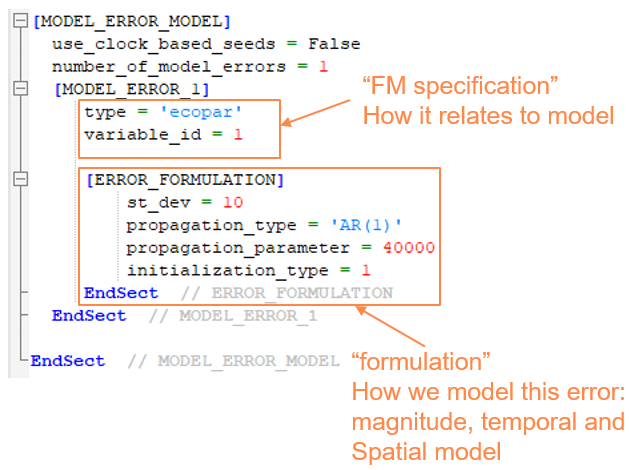
As stated above, the specification of a model error consists of a) the FM specification and b) the error formulation.

The following types of errors are currently supported by the DA module:

Hydrodynamic module HD

Type	Specification	Description	Dim
wlbc	n_bounds = 2 bound_codes = 2, 3	Water level boundary [m]	1d
flowbc	n_bounds = 2 bound_codes = 2, 3	Velocity/flux boundary [m/s]	1d or 2dv
wlbc/flowbc	n_bounds = 2 bound_codes = 2, 3 is_phase_error = true	Boundary phase error [s]	0d
wind	-	u and v wind components [m/s]	2d
windspeed	-	wind speed [m/s]	2d
windphase	-	Wind phase error [s]	0d
HD_parameter	parameter_name = "bed_resistance_coefficient"	Manning (HD2d) or Roughness(HD3d)	2d
HD_parameter	parameter_name = "bed_resistance"	Any type of roughness	2d

Temperature/salinity module TS

Type	Specification	Description	Dim
tempbc	n_bounds = 2 bound_codes = 2, 3	Temperature boundary	1d or 2dv
saltbc	n_bounds = 2 bound_codes = 2, 3	Salinity boundary	1d or 2dv
tempbc/saltbc	n_bounds = 2 bound_codes = 2, 3 is_phase_error = true	Boundary phase error [s]	0d
adsource	component_name = "salinity"/"temperature" source_id = 1	Concentration of source	0d
AD_parameter	component_name = "salinity"/"temperature" parameter_name = "vertical_dispersion_coefficient"	2d perturbation of 3d vertical dispersion	2d
AD_parameter	component_name = "salinity"/"temperature" parameter_name = "vertical_eddy_viscosity_coefficient"	2d perturbation of 3d vertical dispersion	2d
HD_parameter	parameter_name = "light_extinction"	For heat exchange	0d

Transport module TR

Type	Specification	Description	Dim
adbc	n_bounds = 2 bound_codes = 2, 3 component_id = 1	Concentration boundary	1d or 2dv
adbc	n_bounds = 2 bound_codes = 2, 3 component_id = 1 is_phase_error = true	Boundary phase error [s]	0d
adsource	component_id = 1 source_id = 1	Concentration of source	0d
AD_parameter	component_id = 1 parameter_name = "vertical_dispersion_coefficient"	2d perturbation of 3d vertical dispersion	2d
AD_parameter	component_id = 1 parameter_name = "vertical_eddy_viscosity_coefficient"	2d perturbation of 3d vertical dispersion	2d
TR_parameter	component_id = 1	Decay rate	0d

Mud Transport module MT

Type	Specification	Description	Dim
adbc	n_bounds = 2 bound_codes = 2, 3 fraction_id = 1	Concentration boundary	1d or 2dv
adbc	n_bounds = 2 bound_codes = 2, 3 fraction_id = 1 is_phase_error = true	Boundary phase error [s]	0d
adsource	fraction_id = 1 source_id = 1	Concentration of source	0d
AD_parameter	fraction_id = 1 parameter_name = "vertical_dispersion_coefficient"	2d perturbation of 3d vertical dispersion	2d
AD_parameter	fraction_id = 1 parameter_name = "vertical_eddy_viscosity_coefficient"	2d perturbation of 3d vertical dispersion	2d
MT_parameter	parameter_name = settling_velocity fraction_id = 1		2d
MT_parameter	parameter_name = settling_velocity_coefficient fraction_id = 1		2d
MT_parameter	parameter_name = "deposition_critical_shear_stress" fraction_id = 1		2d
MT_parameter	parameter_name = "erosion_critical_shear_stress" fraction_id = 1		2d
MT_parameter	parameter_name = "roughness"	Bottom roughness	2d
MT_dredging	dredger_id = 1 parameter_name = "rate"	Dredging rate	0d
MT_dredging	dredger_id = 1 parameter_name = "spill"	Dredging spill	0d
MT_dredging	dredger_id = 1 parameter_name = "phase"	Dredging phase error [s]	0d

Ecolab module EL

Type	Specification	Description	Dim
adbc	n_bounds = 2 bound_codes = 2, 3 state_variable_id = 1	Concentration boundary	1d or 2dv
adbc	n_bounds = 2 bound_codes = 2, 3 state_variable_id = 1 is_phase_error = true	Boundary phase error [s]	0d
adsource	state_variable_id = 1 source_id = 1	Concentration of source	0d
AD_parameter	state_variable_id = 1 parameter_name = "vertical_dispersion_coefficient"	2d perturbation of 3d vertical dispersion	2d
AD_parameter	state_variable_id = 1 parameter_name = "vertical_eddy_viscosity_coefficient"	2d perturbation of 3d vertical dispersion	2d
EL_constant	constant_id = 1	0d or 2d Ecolab constants	0d or 2d
EL_state_variable	state_variable_id = 1	0d EL variables (only white_noise)	0d
EL_forcing	forcing_id = 1	0d or 2d Ecolab forcing	0d or 2d

Spectral wave module SW

Type	Specification	Description	Dim
wavebc	n_bounds = 2 bound_codes = 2, 3 subtype = "wave_height"	Scaling of total energy [-] (multiplicative) example st_dev: 0.05 (5%)	0d
wavebc	n_bounds = 2 bound_codes = 2, 3 subtype = "wave_period"	Shift of wave periods [s] example st_dev: 0.25	0d
wavebc	n_bounds = 2 bound_codes = 2, 3 subtype = "wave_direction"	Shift of directions [degree] example st_dev: 12.5	0d
wavebc	n_bounds = 2 bound_codes = 2, 3 is_phase_error = true	Boundary time-shift [s] example st_dev: 900.0	0d
wind	-	u and v wind components [m/s] example st_dev: 0.5	2d
windspeed	-	wind speed [m/s] example st_dev: 0.5	2d
windphase	-	Wind time-shift [s] example st_dev: 900.0	0d
SW_parameter	parameter_name = "background_Charnock_parameter"	example st_dev: 0.0005	0d
SW_parameter	parameter_name = "wind_non_dimensional_growth"	beta max example st_dev: 0.05	0d
SW_parameter	parameter_name = "wind_corr_friction_velocity_CAP"	wind CAP ratio of Ufric over U10 example st_dev: 0.005	0d
SW_parameter	parameter_name = "whitecapping_dissipation_cdiss"	Settings:Modifed WAM Cycle 4 example st_dev: 0.3	2d
SW_parameter	parameter_name = "whitecapping_dissipation_delta"	Settings:Modifed WAM Cycle 4 example st_dev: 0.05	2d
SW_parameter	parameter_name = "whitecapping_cds_sat"	Settings:Ardhuin et al example st_dev: 0.000002	0d
SW_parameter	parameter_name = "Nikuradse_roughness"	Bottom friction example st_dev: 0.005	2d

Model error type specification¶

Any type of model error needs to be related to the underlying MIKE FM model. In some cases, this is done simply be specifying the type of the model error in other cases the user needs to supply more information e.g. the id of a FM quantity.

Boundary errors

A MIKE FM model typically has several open boundaries (“bounds”) each having its own unique code (e.g. 3). Often some of these boundaries are adjacent which also means that the errors on these correlates to some extent. To describe this correlation across different boundaries the DA module require the user to specify groups of boundaries. The specification is as follows in a case of a group consisting of two bounds:

[MODEL_ERROR_1] 
    type = 'wlbc'
    n_bounds = 2
    bound_codes = 2, 3
    // (…)

Measurement bias

Measurement bias is a special kind of 0d model error which is used for estimating bias in a particular measurement. The Ensemble Kalman filter assumes that errors in measurements are white---measurement bias can be used if that is not the case.

Error formulation¶

After specifying the model error’s relation to the FM model, we need to specify its formulation in the ERROR_FORMULATION sub-section. The formulation contains the following:

Amplitude and perturbation type (additive, multiplicative, …)
Temporal propagation including initialization
Spatial discretization (horizontal and vertical)
Spatial correlation (horizontal and vertical)

Each of these are explained in detail in the Model error modelling section.

Perturbation type¶

The two basic perturbation types: additive and multiplicative are explained in the Amplitude and perturbation type section. In total, these perturbation_type are available:

additive (default)
additive_non_negative
log_additive
additive_bounded
multiplicative
multiplicative_non_negative
log_multiplicative
multiplicative_bounded

The X_non_negative variants will make sure that the quantity which is perturbed will not be negative after the perturbation (e.g. the wind_speed).

The log_X variants will perform a log-transformation of the quantity to perturbed before doing the perturbation. The inverse log-transform will be performed afterwards. This could be relevant for non-Gaussian quantities e.g. wind speed.

The X_bounded variants require the user to provide perturbation_bounds that the quantity which is perturbed will be enforced to stay within. If your instead wish to bound the value of the perturbation you can set the minimum_value and maximum_value.

Temporal propagation¶

The model error will have a temporal propagation model associated. The following propagation_type are available:

AR(1) – first order autoregressive process (default)
persistence – i.e. no temporal propagation
whitenoise

If the propagation_type is ‘AR(1)’ then a propagation_parameter, which is the process half-life in seconds, must be supplied as well. See ensemble modelling page for an example and experiment with the AR(1) app to get a better understanding of auto-regressive processes.

An initialization_type may be supplied if the propagation_type is not ‘whitenoise’. initialization_type=0 means to start from zero; initialization_type=1 means to start from the specified error amplitude (set by the st_dev).

Horizontal discretization¶

If the model error has a spatial extent (e.g. a boundary or wind error) it needs to be discretized in space. The discretization will typically be coarser than the resolution of the corresponding MIKE FM quantity. The DA engine will perform a (bi-) linear interpolation from the discretized error on to the model quantity before the actual perturbation is done.

Currently three options exist for horizontal_discretization_type of model errors:

0: Constant
1: Linear
2: Equidistant grid

If horizontal_discretization_type=2 then a horizontal_grid_spacing should be provided as well.

Horizontal correlation¶

The spatially distributed errors are in most cases correlated in space. Internally in the code the correlation is described by a covariance matrix Q which describes how the errors co-vary across the domain. The user can control that both by the horizontal discretization (see above section) and more directly by specifying a horizontal_corr length scale (and horizontal_corr_function). A typically value for the horizontal_corr could be 5-10 times larger than the horizontal_grid_spacing.

Experiment with the horizontal correlation app to get a better understanding of correlated errors on an equidistant grid.

Vertical discretization and correlation¶

Some errors, e.g. 2dv boundary errors, may be discretized in the vertical direction using the number_of_layers keyword. The error layers will follow relative vertical coordinates ranging from 0 (=bottom) to 1 (=surface). It is possible to specify specific layer_positions if equidistant layers are not sufficient. The relative vertical coordinate will be applied for the error regardless of the vertical discretization of the model (sigma vs sigma-z).

It is possible to specify vertical_corr_function and vertical_corr in the same way as horizontal correlation. The vertical_corr is also given in meters.

PFS Section `MODEL_ERROR_MODEL`¶

The overall structure of the MODEL_ERROR_MODEL section is:

[MODEL_ERROR_MODEL] 
    number_of_model_errors = 2
    [MODEL_ERROR_1] // (…)
    [MODEL_ERROR_2] // (…)
EndSect

Each of the model errors has first a FM specification part and the and error formulation part. For a wlbc error it could look like this:

[MODEL_ERROR_1] 
    type = ‘wlbc’
    n_bounds = 2
    bound_codes = 2, 3
    [Error_Formulation]
        // (…)
    EndSect // Error_Formulation
EndSect

And the error formulation could look like this:

[Error_Formulation]
    st_dev = 0.05 
    perturbation_type = ‘multiplicative’
    propagation_type = 'AR(1)'
    propagation_parameter = 21600.0
    initialization_type = 0
    horizontal_discretization_type = 2
    horizontal_grid_spacing = 1000.0
    horizontal_corr_function = 1
    horizontal_corr = 10000.0
EndSect // Error_Formulation

Overall specification¶

Keyword	Description	Values
[MODEL_ERROR_MODEL]	Section for specifying all model errors
use_clock_based_seeds	The seed is the starting point of the random number generator used for generating the model errors. If use_clock_based_seeds=true it will be different each time the model is executed. If it is false the same sequence of random numbers will be obtained each time	true/false default: true
random_seed	If use_clock_based_seeds=false, a specific seed (an integer value) can be used for initializing the random number generator such that the same sequence of random numbers are obtained each time	default: 1000000
number_of_model_errors		Default: 0

Hereafter follows the specification of each model error.

Basic model error specification¶

Keyword	Description	Values
[MODEL_ERROR_x]	Section for specifying a single model error
type	type of model error	see table above
n_bounds, bound_codes	specification of water level boundary error if type='wlbc'
module_name, parameter_name, etc...	specification of each type of model will be different - see table above
include_in_state	Should the model error be part of the state vector and thereby be updated upon assimilation?	true/false default: true
name	Optionally, a user-defined name for the model error can be specified.	Default: according to number and type e.g. “err01_wind_u”

Every model error has an Error_Formulation which is defined in a separate section.

Error formulation¶

Amplitude and perturbation type¶

Keyword	Description	Values
Error_Formulation	Section for specifying error formulation
st_dev	Standard deviation of the error
minimum_value	Lower bound of the error (typically not used)	Default: -1e10
maximum_value	Upper bound of the error (typically not used)	Default: 1e10
perturbation_type	How should the FM quantity be modified?	'additive' (default) 'multiplicative' 'additive_non_negative' 'log_additive' 'additive_bounded' 'multiplicative_non_negative' 'log_multiplicative' 'multiplicative_bounded'
perturbation_bounds	For perturbation_type X_bounded vector with minimum and maximum value for the perturbed quantity	Default: -1e10, 1e10

Temporal propagation¶

Keyword	Description	Values
propagation_type	Name of temporal propagation model	'whitenoise' 'presistence' 'AR(1)' (default)
propagation_parameter or propagation_parameters	Parameters for the temporal propagation model	If 'whitenoise' or 'persistance': not used If ‘AR(1)’: half time in sec Default: 21600.0
initialization_type	How should the model error be in the first time step	0: No initialization (start from 0) 1: (start from st_dev) Default: 0

Horizontal discretization and correlation¶

Keyword	Description	Values
horizontal_discretization_type	Type of discretization	0: Horizontally constant 1: (Piecewise) Linear 2: Equidistant grid Default: 2
horizontal_grid_spacing	Grid spacing in meters (only if type=2). Be careful not to set this number too small as it will make the error initialization process extremely slow.	Default: 25% of the average of x- and y- domain lengths
horizontal_corr_function	Correlation function (e.g. Gaussian).	1: Gaussian 2: Exponential 3: Gaspari & Cohn 4: Cubic exponential 5: Cubic polynomial 6: Step Default value: 1
horizontal_corr	Correlation length scale in meters	Default: 10000.0

Vertical discretization and correlation¶

Some errors can also be discretized in the vertical direction, e.g. 2dv boundary errors.

Keyword	Description	Values
number_of_layers	Number of error layers (1=no vertical discretization)	Default: 1
layer_positions	Position of each layer in relative coordinates from 0 (=bottom) to 1 (=top). Must start with 0 and end with 1.	Default: equally distributed between 0 and 1
vertical_corr_function	Correlation function (e.g. Gaussian) for vertical correlation	1: Gaussian 2: Exponential 3: Gaspari & Cohn 4: Cubic exponential 5: Cubic polynomial 6: Step Default value: 1
vertical_corr	Vertical correlation length scale in meters	Default: 100.0

State space¶

Variables and meshes¶

The state vector should contain the prognostic variables of a given model and potentially a few auxiliary variables that are used by the model across timesteps (and are different for the different members).

HD

The state vector of a HD model (mode=2) is populated by setting hd_state_space_type = 1. That is sufficient in most applications but if the user would like fine-grained control over what should be included in the state vector it can be done by setting the type_x parameters shown below (here shown with default values). See table below for the possible options.

[MODEL_STATE_SPACE]  
    hd_state_space_type = 1
    type_surface = 1
    type_velocity = 1
    type_flux = 0 
    type_temperature = 1
    type_salinity = 1
    type_turbulence = 1
EndSect

TR

The state vector of a decoupled TR model will be populated by setting tr_state_space_type = 1. The hd_state_space_type should be 0 (or not set) since the HD field is read as a forcing in the decoupled mode. In a coupled model both should be 1.

MT

The state vector of a decoupled MT model will be populated by setting mt_state_space_type = 1. The hd_state_space_type should be 0 (or not set) since the HD field is read as a forcing in the decoupled mode. In a coupled model both should be 1.

EL

The state vector of a decoupled EL model will be populated by setting el_state_space_type = 1. The hd_state_space_type should be 0 (or not set) since the HD field is read as a forcing in the decoupled mode. In a coupled model both should be 1.

SW

The action density 'SW%a' is the only prognostic variable in the spectral wave module. It belongs to the “spectrum” mesh

[MODEL_STATE_SPACE]  
    sw_state_space_type = 1 
    type_Hm0 = 1
    type_Tp = 0
    type_MWD = 0
    type_windspeed = 1 
EndSect

Variable names and id¶

A list of all variables (id, name and size) will be outputted to the log file in the setup phase of the simulation (MODEL_STATE_SPACE section). It could like this:

============== Model/error variables included in state ===============

     -------------------------------------------------------
      var type     id                name     size   ndim
     -------------------------------------------------------
      model-var:    1                HD%s     3992     2
      model-var:    2                HD%u    41400     3
      model-var:    3                HD%v    41400     3
      model-var:    4                HD%w    41400     3
      model-var:    5               HD%ws    41400     3
      model-var:    6             TS%temp    41400     3
      model-var:    7             TS%salt    41400     3
      model-var:    8               KE%tk    41400     3
      model-var:    9               KE%ep    41400     3
      error-var:   10          err01_wlbc        2     1

Variable Transformation¶

Non-gaussian variables---e.g. significant wave height Hm0---may be log-transformed before and after the assimilation for better performance. The same transformation will be applied to the measurement of the same variable. Note that the measurement error description will now also be in the transformed space - so you may want to reconsider the st.dev of the measurement error. It does not make sense to transform variables which are not used for assimilation.

[MODEL_STATE_SPACE]  
    // (…)    
    number_of_variable_transforms = 1
    [VARIABLE_TRANSFORM_1] 
        variable_name = "SW%Hm0"
        transform_type = 1   // 1=log, 2=square, -1=exp, -2=sqrt
    EndSect
EndSect

Consult the log file (MODEL_STATE_SPACE section) of an initial simulation to obtain the variable_name of the variable you wish to transform.

PFS Section `MODEL_STATE_SPACE`¶

[MODEL_STATE_SPACE]  
    hd_state_space_type = 0
    type_surface = 0
    type_velocity = 0
    type_flux = 0 
    type_temperature = 0
    type_salinity = 0 
    type_turbulence = 0

    tr_state_space_type = 0
    mt_state_space_type = 0
    el_state_space_type = 0
    sw_state_space_type = 0

    sw_state_space_type = 1 
    type_Hm0 = 1
    type_Tp = 0
    type_MWD = 0
    type_windspeed = 1 

    number_of_variable_transforms = 1
    [VARIABLE_TRANSFORM_1] 
        variable_name = "SW%Hm0"
        transform_type = 1
    EndSect
EndSect  // MODEL_STATE_SPACE

HD

Keyword	Description	Values
hd_state_space_type	HD model	0: not included 1: included
type_surface	Type of state variable for the free surface	0: not included 1:s (surface elev) (default) 2:h (total water depth)
type_velocity	Type of state variables for the velocity components	0: not included 1:u,v,w,ws, (default) 2:hu,hv,hw,hws
type_flux		0: not included (default) 1: included
type_temperature		0: not included 1: included (default)
type_salinity		0: not included 1: included (default)
type_turbulence		0: not included 1: included (default)

TR, MT and EL

Keyword	Description	Values
tr_state_space_type		0: not included 1: included
mt_state_space_type		0: not included 1: included
el_state_space_type		0: not included 1: included

SW

Keyword	Description	Values
sw_state_space_type		0: not included 1: included
type_Hm0	Significant wave height	0: not included 1: included (default)
type_Tp	Peak period	0: not included (default) 1: included
type_MWD	Mean wave direction	0: not included (default) 1: included
type_windspeed		0: not included (default) 1: included

Variable Transforms

Keyword	Description	Values
number_of_variable_transforms	Number of variables that should be transformed	Default 0
VARIABLE_TRANSFORM_x	Section for a specification of a single variable transformation
variable_name	Variable name for variable that should be transformed.	Default: ''
transform_type	Type of transformation	0: no transformation (=deactivated) 1: log-transform 2: square-transform

Nudging¶

Full-field nudging of a variable (typically from another model) is possible for any DA type. It is activated if the [NUDGING] is present. The technique, which blends the computed solution of a variable (e.g. salinity) with data provided from a file, can be used for maintaining long term deep ocean solutions. It can be combined with any type of data assimilation.

Let $f$ denote a vector of values for a single variable (e.g. salinity) at a given time step. The nudging now blends the computed solution $f_{FM}$ with the inputted values $f_{input}$ by the nudging factor $\alpha$ :

$f = (1- \alpha) f_{FM} + \alpha f_{input} = f_{FM} + \alpha (f_{input}-f_{FM})$

The factor $\alpha$ may be supplied either directly or as "half-life" $\tau$ making it independent of the nudging time step (=assimilation time step) $dt$ by this relation

$\alpha = 0.5^{dt/\tau}$

The factor $\alpha$ can be a constant (format 0) or provided as a "map" (format 2) with the same spatial dimensions as the values.

The nudging section also allows for directly specifying an update for a given variable by setting the is_update switch to true in which case $f$ is updated by

$f = f_{FM} + \alpha_m f_{input}$

In which case the factor $\alpha_m$ is a moderation factor.

Note

Full-field nudging was introduced with MIKE Zero 2021 as a subsection of [METHOD]. For MIKE Zero 2021 update 1, it has been moved to it's own section.

PFS Section `NUDGING`¶

[NUDGING]
    number_of_inputs = 1
    [INPUT_1]
        variable_name = 'salinity'
        file_name = |.\data\salinity_from_CMEMS.dfsu|
        item_number_values = 1 

        factor_type = 2   // 1:plain factor or 2:half-life
        factor_format = 0
        // file_name_factor = |.\data\nudging_factor_map.dfsu|
        // item_number_factor = 2            
        factor = 1200   // half-life in seconds if factor_type=2
    EndSect // INPUT_1 
EndSect // NUDGING

The NUDGING section may also be used for directly providing an update on a single variable if the switch is_update is to true.

    [INPUT_1]
        variable_name = 'surface elevation'
        is_update = true
        moderation_factor = 1.0
        file_name = |.\data\StateUpdate_area.dfsu|
        item_number_values = 1 
    EndSect // INPUT_1

Keyword	Description	Values
[NUDGING]	Section for specifying full field nudging
number_of_inputs	Number of input files	Default value: 0
[INPUT_x]	Section for specifying Nudging for a single input field (and variable)
variable_name	Name of this variable (must be in state)	Default value: ''
file_name	File with data	Default value: ''
item_number_values	Item number of data to be used for nudging	Default value: 1
factor_format	Is the factor a constant (0) or a map (2)	Default value: 0
factor_type	Should the factor be given as direct blending factor (1) or as a half time (2)	Default value: 1
factor	If factor_format=0, then this constant factor will be used.	Default value: 0.2 or 1800s (if factor_type=2)
file_name_factor	File with factor (if factor_format=2)	Default value: ''
item_number_factor	Item number of nudging factor in factor file	Default value: 1
is_update	Use standard nudging blending computed and inputted field (false) or simply add input to computed solution (true)	Default value: false
moderation_factor	If is_update=true. This factor is for reducing the effect of the update. If set to 1 then the update will done fully, if 0.9 then only 90%.	Default value: 1.0
type_of_space_interpolation	Should the values be spatially interpolated when read from disk? Not needed if the same mesh is used.	0: no interpolation 1: linear interpolation Default value: 0 (off)

Measurements¶

The EnKF assumes that measurements are mutually independent and that the measurement errors are gaussian distributed and non-correlated in time.

Types of measurements¶

Different model quantities can be observed depending on the type of model

HD
- Water level (2d)
- ua, va (2d)
- u, v (3d)
TS
- salinity
- temperature
TR
- e.g. TR%COMPONENT_2
MT
- e.g. MT%SSC_FRACTION_1
EL
- e.g. EL%STATE_VARIABLE_3
SW
- Significant wave height

In terms of data file types, the following types are supported:

Fixed position station data (scalar) in dfs0 (type 1)
Track data in dfs0 with first two items as x,y-coordinates (type 2)
Horizontal grid data in dfs2 (type 3)
Horizontal flexible mesh data in dfsu2d (type 4)
Vertical column data as multiple items in dfs0 (type 5)

Station measurements¶

Type 1. Station measurements are fixed position scalar measurements relating to a single observable variable in the FM model. The data is supplied in a dfs0 file and the user needs to provide the following information:

Measured variable
File name and item number
Position of the measurement
St.dev (=the level of error in the measurement – see section below)

3D measurements

If the observed quantity is a 3d field (e.g. salinity), the user needs to provide the z-coordinate as well. Note that a specific layer is found in the model initialization phase with surface level as specified by the initial condition. It does not change dynamically during the simulation.

Track measurements¶

Type 2. Track measurements are scalar measurements with changing position relating to a single observable variable in the FM model – it could be altimeter SSH data from a satellite. The data is provided in a dfs0 file in which the two first items are the x,y-coordinates. The user needs to provide the following information:

Measured variable
File name and item number of the data (x,y-coordinates are the first two items)
St.dev (=the level of error in the measurement – see section below)
Error correlation along track

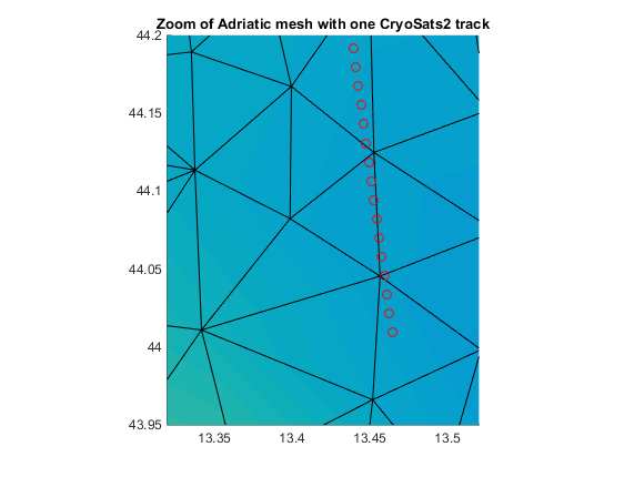
Chart shows an example of a track measurement on top of a MIKE FM mesh

NOTE: 3D track measurements are not yet supported

Horizontal grid measurements (raster)¶

Type 3. Horizontal grid measurements are vector measurements with fixed positions relating to a single observable variable in the FM model – it could be gridded Chlorophyll maps obtained from satellite. The data is provided in a dfs2 file which contains the geographical specification of the measured points. The user needs to provide the following information:

Measured variable
File name and item number of the data (x,y-coordinates are read from dfs file)
St.dev (=the level of error in the measurement – see section below)
Error correlation

NOTE: dfs1 and dfs3 are not yet supported.

Flexible mesh measurements (horizontal)¶

Type 4. Unstructured (dfsu) measurements are vector measurements with fixed positions relating to a single observable variable in the FM model. The mesh of the measurement can be the same or different to the model mesh. The data is provided in a dfsu file which contains the geographical specification of the measured points. The user needs to provide the following information:

Measured variable
File name and item number of the data (x,y-coordinates are read from dfsu file)
St.dev (=the level of error in the measurement – see section below)
Error correlation

NOTE: dfsu files with vertical data (3d or 2dv) are not yet supported.

Vertical column measurements¶

Type 5. Vertical column measurements can be provided as multiple-item dfs0 where the different items represent different depths. Dfs0 files are chosen over dfs1 as the depths often will be non-equidistant which is not easily handled with dfs1 files. Both the horizontal and vertical positions needs to be provided by the user. The following information should be provided:

Measured variable
File name and item numbers of the data
Horizontal position of the column
Vertical positions (depths) corresponding to each of the items
St.dev (=the level of error in the measurement – see section below)
Vertical error correlation (optional)

Observation operator and relation to model¶

After the observed data have been read from file it needs to be related to model:

which variable have been measured?
At what time should the data be used?
Where in the model is the observation located?
And should neighbouring cells also be taken into account as well?

Measurement errors

A good specification of the measurement errors is essential to the performance of the data assimilation scheme.

The errors description should account for both:

Instrumentation/acquisition errors
Representation errors

The first type is relatively easy to understand - what is the accuracy of a certain sensor e.g. on a satellite. The representation error has to do with how well the model can represent an observable quantity which is a consequence of model equations, numerical techniques, parametrizations and discretization. As an example, a tide gauge in a harbour may determine the surface elevation very accurately but if harbour resonance is recorded by the sensor and the model is a regional model it will not include a description of harbour resonance or other local scale effects. That is representation error.

Varying measurement errors

In some cases, measurement errors vary in time (e.g. may be larger for larger values) or vary in space (e.g. satellite data may have different errors close to land than at open sea).
It is possible to provide spatially and/or temporally varying errors as an item 'item_number_stdev' in the dfs data file. The values will be interpolated in time the same way as the actual observation data. If values are missing or below 1e-7, the default value for st_dev will be applied.

Correlation of measurement errors

It can be quite difficult to determine the correlation between errors e.g. along an altimeter track.

NOTE: it is not possible to set the correlation function yet. It is hard-coded to the exponential function.

Maximum innovation¶

The measurement-model difference in the observation position is called innovation. If the measurement is very different from the model (e.g. erroneous data point) then the data assimilation update may become radical and could potentially lead to model blow up or other unwanted effects. The user have the possibility to disregard measurement points with values that result in absolute innovation which is larger than a specified threshold called max_abs_innovation_point. This is a point-wise assessment.

A similar threshold can be set on the mean of the absolute innovation of a batch of points (e.g. points in a track measurement within one time step) by max_mean_abs_innovation_batch. This assessment will only be done in case of multiple points in the same measurement in a timestep and only on the points which has not been disregarded due to the point-wise test using max_abs_innovation_point.

If measurement points (or batches of points) are discarded a message will be printed in the log file.

PFS Section `MEASUREMENTS`¶

[MEASUREMENTS]
    number_of_independent_measurements = 1

    [MEASUREMENT_1]
        include = 1
        name = 'ts_WL_NW'

        type = 1         
        file_name = |.\..\Measurements\ts_WL_NW.dfs0|
        item_number = 1 
        item_number_stdev = 2
        data_offset = 0.0 

        measured_variable = 'water level'
        type_time_interpolation = 1
        time_window_in_seconds = 300
        position = 251, 752
        coordinate_type = 'NON-UTM'         
        type_of_space_interpolation = 1

        st_dev = 0.01
        error_temporal_corr = 1 
        error_horizontal_corr = 1
        max_abs_innovation_point = 0.30

        group = 1  
    EndSect
EndSect

For a simple station measurement the following will suffice in most cases:

[MEASUREMENT_1]
    include = 1
    name = 'ts_WL_NW'

    type = 1
    measured_variable = 'water level'

    file_name = |.\..\Measurements\ts_WL_NW.dfs0|
    item_number = 1 
    position = 251, 752

    st_dev = 0.01   
    max_abs_innovation_point = 0.30 
    group = 1  
EndSect

A typical track measurement would look like this:

[MEASUREMENT_1]
    include = 1
    name = 'track A'

    type = 2
    measured_variable = 'water level'

    file_name = |.\..\Measurements\track_A.dfs0|
    item_number = 3 

    st_dev = 0.03
    error_horizontal_corr = 300    
    max_abs_innovation_point = 0.40    
    time_window_in_seconds = 300
EndSect

A typical horizontal grid (raster) measurement could be specified like this:

[MEASUREMENT_1]
    include = 1
    name = 'Raster'

    type = 3
    measured_variable = 'EL%STATE_VARIABLE_1'

    file_name = |.\obs\BOD.dfs2|
    item_number = 1

    st_dev = 1.0
    type_of_space_interpolation = 0
    time_window_in_seconds = 1800
EndSect

A typical vertical column measurement would look like this:

[MEASUREMENT_1]
    include = 1
    name = 'Column B'
    type = 5
    measured_variable = 'u' 
    horizontal_position = 150, 150

    file_name = |.\..\Measurements\column_B.dfs0|
    number_of_items = 6
    item_numbers = 1, 2, 3, 4, 5, 6
    vertical_positions = -200, -150, -100, -80, -60, -40
    type_of_spatial_interpolation = 1

    st_dev = 0.02
    error_vertical_corr = 200
EndSect

Basic specification

Keyword	Description	Values
include	Should this measurement be included for data assimilation, only for validation or not at all?	0: not included 1: used for assimilation 2: used only for validation Default: 1
name	User-defined name for this measurement (optional)	Default: e.g. Meas001

Data file specification

Keyword	Description	Values
type	Type of measurement data file	1: fixed station series (dfs0) 2: track time series (dfs0) 3: fixed gridded data (dfs2) 4: fixed unstruct data (dfsu) 5: vertical column (dfs0) Default: 1
file_name	Path of the data file
item_number	Which item in the file contains the data (note that for track data files it is assumed that the x,y coordinates are the two first items) (type 1-4)	Default: 1
item_number_stdev	Which item in the file contains the measurement error (described as standard deviation)? (type 1-4)	Default: 0 (inactive)
number_of_items	In vertical column data files, how many items/depths does the file contain (type 5 only)	Default: 1
item_numbers	Which items in the file contains the vertical column data (type 5 only)	Default: 1
data_offset	Add this amount to all data in file	Default: 0.0

FM model specification

How do the observations relate to the model: what variable? at what times? in what positions?

Keyword	Description	Values
measured_variable	Which of the MIKE FM model variables are being measured	See variable list Default: ‘water level’
type_time_interpolation	If type not 2: When should the model consider the measurement?	0: no interpolation 1: linear interpolation 2: cubic spline interp. Default: 1
time_window_in_seconds	If type_time_interpolation is 0 you can add a “window” around the observation time.
position	Where spatially in the model is the observation? (type 1)	x,y,z coordinate of measurement
horizontal_position	Where horizontally in the model is the vertical col. observation? (type 5)	x,y coordinate of vertical col.
coordinate_type	Optionally. If the position is given in another coordinate system than the model.	Default: model default
vertical_position	At what depths are the vertical column observations? (type 5)	z coordinate of vertical col.
type_of_spatial_interpolation	Should the observation operator only refer to the cell the observation is located in (0) or should it be a weighted average between the cell and its neighbours (1 or 2)	0: no interpolation 1: linear interpolation 2: inv dist weight. (neighbours) Default: 1

Specification of measurement errors

Keyword	Description	Values
st_dev	What is the average measurement error (see also item_number_stdev above)	Default: 0.1
error_temporal_corr	Correlation time in seconds (only track measurements - type 2)	Default: 0 (no correlation)
error_horizontal_corr	Correlation length scale in meters (2d measurements - type 3 and 4)	Default: 0 (no correlation)
error_vertical_corr	Correlation length scale in meters (vertical column measurements - type 5)	Default: 0 (no correlation)
max_error_corr	Limit correlation of meas errors for numerical reasons. Model may be become unstable if this value is set too high.	>=0 and <=1 Default: 0.85 (no correlation)
Rinv_singular_values_cutoff	When doing the pseudo-inverse of R where should we apply the (relative) cut-off on the singular values	>=0 and <=1 typical 0.001--0.1 Default: 0.001

Specification of maximum measurement-model difference

Keyword	Description	Values
max_abs_innovation_point	Measurement points with values that result in innovation (model-measurement difference in observation point) which is the absolute value is larger than this threshold will be disregarded	Default: 1e10 (off)
max_mean_abs_innovation_batch	Measurements consisting of several points in a time step (e.g. satellite track) with values that gives a mean absolute innovation (model-measurement abs. difference as mean over all points in a batch/timestep) larger than this threshold will be disregarded	Default: 1e10 (off)

Localization

Keyword	Description	Values
group	Group number of this measurement used for assigning per-group localization settings.	Default: 1

Estimator (and regularization)¶

The EnKF approximates the “true” error covariance by the sample error covariance by the ensemble representation. The limited size of the ensemble inevitably introduces noise which increases with decreasing ensemble size. The noise is evident both in spatial and temporal directions.

The spatial noise in the error covariance often referred to as spurious long-range correlations may be accounted for by so-called localisation, where the effect of the update is decreased gradually away from the point of observation by multiplying by a taper function. In the Serial ESRF, this can be conveniently done directly on the error covariance P (called covariance localisation CL). In the ETKF and DEnKF, the so-called Local Analysis (LA) performs the localisation by element-by-element formulation of the update equations.

Smoothing in the serial ESRF¶

The EnKF approximates the “true” error covariance by the sample error covariance using an ensemble representation. The limited size of the ensemble inevitably introduces noise that increases with decreasing ensemble size. The noise is evident both in spatial and temporal directions. In this report, we are concerned only with the temporal behavior.

If the observations are scalar and fixed in space (like tide gauge stations), the Serial ESRF gives us the opportunity to reduce the noise in the temporal direction by smoothing the error covariance exponentially with a smoothing factor s with

$P_{sm}^k = s P^k + (1-s) P_{sm}^{(k-1)}, \qquad \qquad s \in [0;1]$

which is a good approximation for slowly-varying error covariance. In practice for tidal and storm surge models, smoothing of the error covariance allows for the use of much smaller ensemble e.g. 8 instead of 50. The choice of smoothing factor becomes a tuning parameter and a compromise between a reduction of high-frequency error covariance noise and maintaining the EnKF’s ability to adapt dynamically to new situations. The smoothing factor s is determined from desired half time $\tau$ and the time step length $\Delta t$ by the relation

$s = 1 - 0.5^{\frac{\Delta t}{\tau} }$

In practical coastal-ocean applications, a smoothing factor corresponding to a 3-hour half time has shown to be a good choice. If the time step $\Delta t$ 5 minutes, then the smoothing factor amounts to s = 0.0191. The figure below shows the relative weights for the previous time steps with these values.

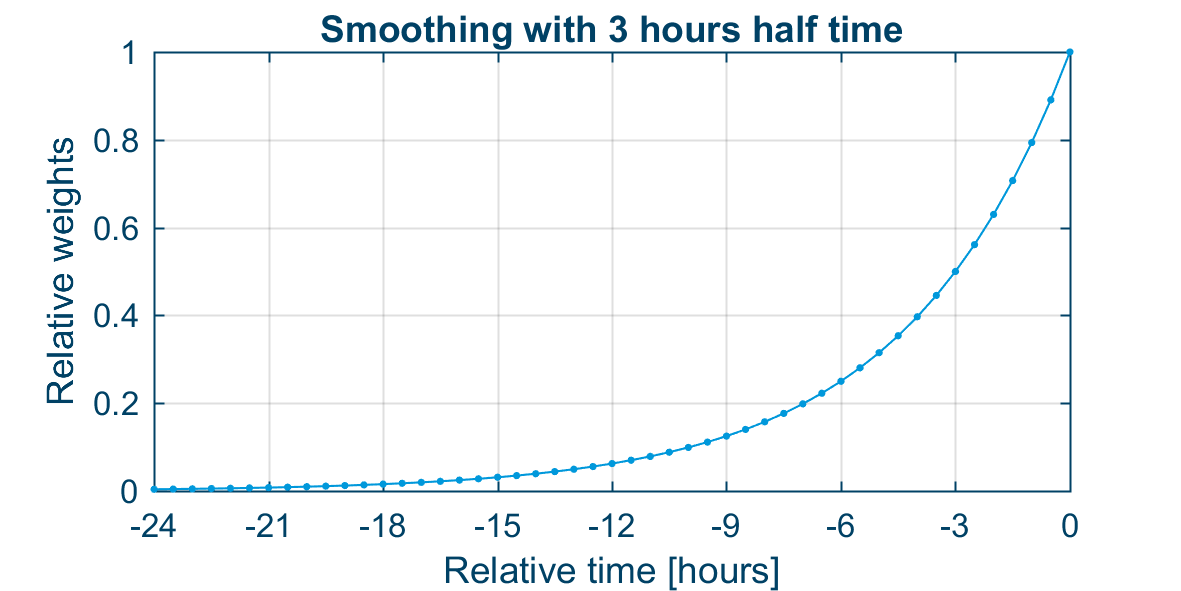
Relative weights of first order smoothing for previous hours with time step $\Delta t = 5$ minutes and half time $\tau = 3$ hours.

The figure below shows time series of three different error covariances. Notice how noisy the 8 member $P_m$ appears and how much better the smoothed 8 members $P_{smooth}$ becomes. Smoothing inevitably introduces a time lag as it uses information from previous time steps, which the figure also reveals.

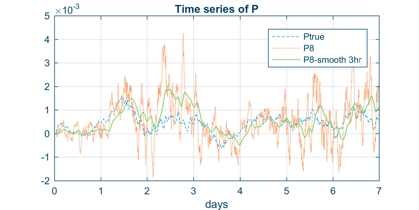
Time series of three different error covariances: the converged $P_{true}$ , a noisy 8 member $P_m$ and a 3-hour smoothed $P_{smooth}$ also with 8 members.

Random anomaly tail smoothing (RAT)¶

Only the serial ESRF allows us to use direct smoothing of the error covariance $P$ since $P$ is saved for the (few) positions where we need it. This is not generally possible. One way to implement a smoothing technique in an ESRF which does not rely on a few fixed measurement stations would be to keep all previous anomaly vectors to be able to construct the anomaly matrix and thereby smoothed error covariance matrix anywhere and at any time. This, however, would require huge amounts of storage and massive computational powers in the analysis step. Furthermore, many anomaly vectors would be linearly dependent (unless the time steps are large) and weights would be vanishing small far away from the current time step anyway. This is clearly not a realistic path to follow.

Another idea is to instead keep only a reduced number $m_{tail}$ of “old” anomaly vectors in an anomaly tail $A_{tail}$ . At each time step, we update the anomaly tail by replacing $m_{rep}$ random anomaly vectors with $m_{rep}$ random vectors from the dynamic anomaly matrix $A_{dyn}$ . The dynamic anomaly matrix is here simply the normal anomaly matrix, but named “dynamic” to distinguish it from the anomaly tail.

We define also the hybrid anomaly matrix A consisting of both the dynamic anomaly matrix $A_{dyn}$ with m_d members and the anomaly tail $A_{tail}$ with $m_{tail}$ members in the following way

$A=[\alpha_{dyn} A_{dyn} │\alpha_{tail} A_{tail} ], \qquad \alpha_{dyn}=\sqrt{\frac{\beta (m-1)}{m_{dyn} - 1}}, \qquad \alpha_{tail}=\sqrt{\frac{(1-\beta) (m-1)}{m_{tail} - 1}}$

This new temporal smoothing technique is called Random Anomaly Tail abbreviated RAT. Notice that the technique contains three tuning parameters:

the number of vectors in the tail $m_{tail}$ ,
the number of replacements pr step $m_{rep}$ , and
the weighting factor $\beta$ between the dynamic anomaly matrix and the anomaly tail.

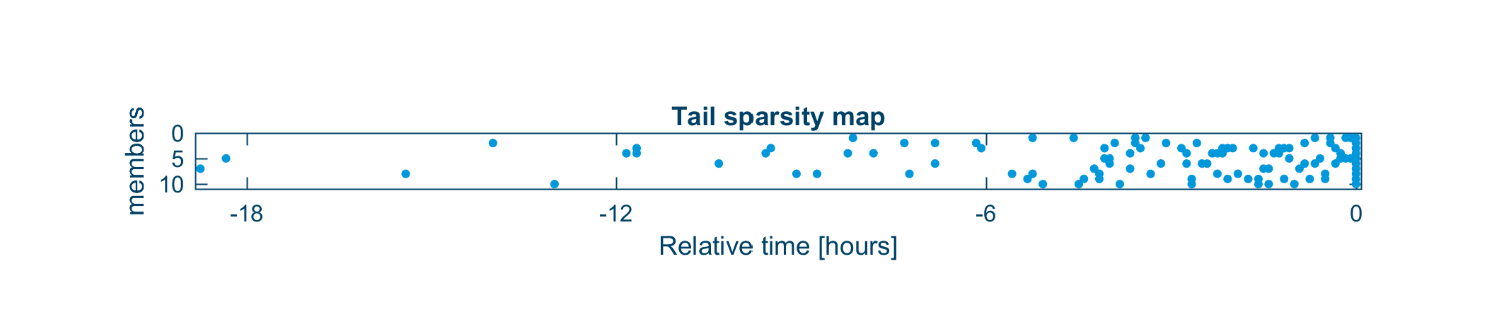
An example of a sparsity map from RAT smoothing with $m=10$ , $m_{tail}=100$ , and $m_{rep}=2$ showing a dot for each anomaly vector in a timestep-vs-member coordinate system.

By collecting these randomly picked anomaly vectors in 1-hour bins (12 time steps) and multiplying with the relevant weight ( $\beta$ or $(1-\beta )$ ), we can express the same data as relative weights as seen in the figure below. Notice how the distribution of the anomaly tail stochastically approximates the 3-hour smoothing from the figure shown above.

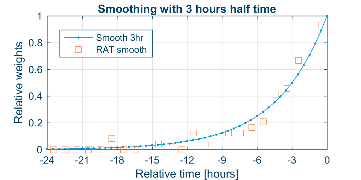
An example of relative weights from RAT smoothing aggregated in 1-hour bins and plotted on top of the standard 3-hour smoothing. The aggregated RAT weights are from the same case as shown on the figure above with $m=10$ , $m_{tail}=100$ , and $m_{rep}=2$ .

Advice on parameters¶

The amount of smoothing to be used in a given DA model is dependent on the dynamics of the model and the typical time scales of the underlying system. As already mentioned, for many coastal-ocean models that include tides, a good practical choice is 3-hour smoothing. And typically, if one is concerned mainly with water levels, then 8 members would give quite good results with this amount of smoothing.

The new RAT smoothing has three tuning parameters $m_{tail}$ , $m_{rep}$ and $\beta$ . Considering similar types of coastal-ocean applications, the following settings seem to lead to best results with moderate number of members m with 8 < m < 15:

Parameter	min	max	Comment
$m_{tail}$	5m	15m	More tail members give more smoothing (but is also computational expensive). Increasing the number seems to have a significant positive effect especially if m is small (e.g. m<10).
$m_{rep}$	1	2	Few replacements will give longer tail (and more smoothing); use $m_{rep}$ =1 if m<10
$\beta$	0.01	0.4	0.1 seems like a good practical choice. Larger value means more smoothing.

To resemble 3-hour smoothing with m=8 members, it is suggested to use $m_{tail}=100$ , $m_{rep}=1$ and $\beta =0.1$ . Note below that the smoothing_tail_weight equals $(1 - \beta )$ .

PFS Section `ESTIMATOR`¶

[ESTIMATOR]
    type = 1
    [REGULARIZATION]
        use_temporal_smoothing = false
        smoothing_halftime = 21600
        use_localization = false
        [LOCALIZATION] 
            number_of_groups = 1
            [GROUP_1]
                horizontal_corr_function = 3
                horizontal_corr = 200000
                vertical_corr_function = 3
                vertical_corr = 150
            EndSect  // GROUP_1
        EndSect  // LOCALIZATION
    EndSect  // REGULARIZATION
EndSect

Smoothing¶

The smoothing of the error covariance is relevant for EnKF models (type 1). The technique is different for the serial algorithm (algorithm 1) and the transform-algorithms (algorithm 2 and 3).

Keyword	Description	Values
use_temporal_smoothing	Should the error covariance smoothing be activated?	Default: false
smoothing_halftime	If algorithm=1: Half-life in seconds for the first order smoothing filter applied to the error covariance	Default: 0 (=off)

Using RAT smoothing (algorithm 2 or 3), the following parameters will instead need to be specified (see above section for advice on parameters):

Keyword	Description	Values
smoothing_tail_size	How many “old” ensemble anomalies should be stored in the tail.	Default: 100
smoothing_tail_weight	How much should the tail be weighted relative to anomalies of the current time step? smoothing_tail_weight = $1- \beta$	Default: 0.8
smoothing_num_re placements_pr_step	How many ensemble anomalies should be replaced in the tail in each time step (use 1 or 2)	Default: 2

Localization¶

The localization works on groups of measurements. When a measurement is defined it can be assigned a group id by the user (see Measurements ). Localization settings can now be controlled for each group individually in the LOCALIZATION section.

Keyword	Description	Values
use_localization		Default: false
LOCALIZATION	Section for specifying localization (spatial regularization)
number_of_groups	Number of measurement groups for which the localization will be defined.
GROUP_x	Section for specifying localization for a specific measurement group
horizontal_corr_function	Correlation function (e.g. Gaussian) to be used for distance-based tapering	1: Gaussian 2: Exponential 3: Gaspari & Cohn 4: Cubic exponential 5: Cubic polynomial 6: Step Default value: 3
horizontal_corr	The horizontal correlation length scale in metres	Default: 100000
vertical_corr_function	Correlation function (e.g. Gaussian) to be used for vertical distance-based tapering (3d models only)	1: Gaussian 2: Exponential 3: Gaspari & Cohn 4: Cubic exponential 5: Cubic polynomial 6: Step Default value: 3
vertical_corr	The vertical correlation length scale in metres (3d models only)	Default: 10000000 (=full)

ErrCovIO¶

ErrCovIO is short for Error Covariance Input-Output. If only fixed station measurements have been used in an EnKF simulation (DA type=1) the error covariance matrix for the measurement station positions for all model variables can be outputted to disk. This is only possible if DA type=1 and algorithm=1 (serial EnKF algorithm) is selected.

The stored error covariance matrices can be read by the DA model in a so-called steady run (DA type=3) which requires only one model instance (not an ensemble model). See also Steady.

Specifying the error covariance input and output is done in the [ERRCOV_IO] section.

Error covariance files and file names¶

Model variables will be outputted to files according to the field type. Water level in an 3d HD model will as example be outputted to a 2d “area” file whereas velocities will be outputted to 3d “volume” file.

For HD/TR/MT/EL models the following file names (dfsu) need to be specified:

File_name_area
File_name_volume (only if 3d model)

For SW models the following file names (dfsu) need to be specified:

File_name_area
File_name_spectrum

Error variables (model errors) will be outputted to separate files (one file per model error)

File_name_[model_error_name]

Where the model error name is the one specified in the corresponding model error section or the default model error name according to type. The file type will be dfs0, dfs1 or dfs2 according to dimension and discretization of the model error.

Error covariance output¶

If the simulation is EnKF (DA type=1) with algorithm 1, the error covariance can be saved to file in the [OUTPUTS] subsection of [ERRCOV_IO]. It is possible to specify any number of error covariance outputs. For each of outputs the following needs to be specified:

Include or not
Time stepping: first and last time step and step factor
Time average or not
Output the smoothen error covariance (see Regularization) or not
Relevant file names

Error covariance input¶

If the simulation is a steady run (DA type=3), the error covariance needs to be loaded from file in the [INPUT] subsection of [ERRCOV_IO]. The following needs to be specified:

include (active or not)
Is the input time averaged or not?
Relevant file names

Note: non time-averaged error covariance inputs are not currently supported. It will give an error if you try.

Note: the number and sequence of measurements needs to fit for the steady run (which reads the error covariance input) and the previously run ensemble model which created the error covariance outputs.

Use cases¶

Error covariance input/output and the various settings can be used for a number of different use cases:

In EnKF run mode (DA type 1, only algorithm 1):

INPUT (not possible)
OUTPUTS
- discrete times (time_average=false)
  - normal (smoothed_out=false)
    - time varying for diagnostics
  - smoothed (smoothed_out=true; only if smoothing is active!)
    - time varying for diagnostics
    - hot-out (last time step) for input in continued EnKF run
- time-averaged (time_average=true, smoothed_out=false)
  - Over (almost) whole simulation (to be used in steady simulation)
  - (over time intervals)

In steady run mode (DA type 3):

INPUT
- read time-invariant input (otherwise error)
OUTPUTS: not possible

PFS Section `ERRCOV_IO`¶

The overall structure of the ERRCOV_IO section is as follows:

[ERRCOV_IO]

    [INPUT]
    EndSect  // INPUT

    [OUTPUTS]
        number_of_outputs = 2
        [OUTPUT_1]  // (...)
        [OUTPUT_2]  // (...)
    EndSect  // OUTPUTS

EndSect

Error covariance input¶

[INPUT]
    include = 1
    time_average = true

    file_name_area = |.\input\ErrCovIO_avg_Area.dfsu|
    file_name_volume = |.\input\ErrCovIO_avg_Volume.dfsu|
    file_name_err01_wind_u = |.\input\ErrCovIO_avg_Wind_err_u.dfs2|
    file_name_err01_wind_v = |.\input\ErrCovIO_avg_Wind_err_v.dfs2|
EndSect

Keyword	Description	Values
INPUT	Section for specifying error cov input
include	Is the input active (1) or not (0)?	0: not active 1: active Default: 0
time_average	Is the input time-averaged?	true/false Default: true
file_name_x	File names of the input files according to the model and error variables selected

Error covariance output¶

[OUTPUT_1]
    include = 1  
    first_time_step = 0
    last_time_step = 360
    time_step_frequency = 360
    time_average = true
    smoothed_out = false

    file_name_area = 'ErrCovIO_avg_Area.dfsu'
    file_name_volume = 'ErrCovIO_avg_Volume.dfsu'
    file_name_err01_wind_u = 'ErrCovIO_avg_Wind_err_u.dfs2'
    file_name_err01_wind_v = 'ErrCovIO_avg_Wind_err_v.dfs2'
EndSect

Keyword	Description	Values
OUTPUT_x	Section for specifying a single error cov output
include	Should this output be active?	0: not included 1: included Default: 1
first_time_Step	First time step (relative to the model overall time stepping) of the output	Default: DA-start
last_time_step	Last time step (relative to the model overall time stepping) of the output	Default: DA-end
time_step_frequency	Time step factor relative to the model overall time stepping	Default: start-end (1 step)
time_average	Should the values be time-averaged over each step (true) or instantaneous (false)	true/false Default: true
smoothed_out	If smoothing is active: should the smoothened error covariance (true) or the instantaneous error covariance be outputted (false)	true/false Default: false
file_name_x	File names of the output files according to the model and error variables selected

EnsembleIO¶

The state vector for all ensemble members can be outputted to disk in the ENSEMBLE_IO section. Likewise, the DA model can read the state vectors to “hot start” a DA model.

Ensemble files and file names¶

Model variables will be outputted to files according to the field type.

For HD/TR/MT/EL models the following file names (dfsu) need to be specified:

File_name_area
File_name_volume (only if 3d model)

For SW models the following file names (dfsu) need to be specified:

File_name_area
File_name_spectrum

Error variables (model errors) will be outputted to separate files

File_name_[model_error_name]

Where the model error name is the one specified in the corresponding model error section or the default model error name according to type. The file type will be dfs0, dfs1 or dfs2 according to dimension and discretization of the model error.

Note that the file name PFS keywords for the Ensemble IO is identical to those for ERRCOV_IO.

It is possible to exclude model variables or model errors in the output if you wish. You do this by setting one of these to false:

include_model_variables = true/false
include_model_errors = true/false

StateUpdate¶

All assimilation models allow the user to output the mean update enforced during the assimilation step (the "increment") for all state variables. This is very useful for assessing the performance of the assimilation scheme. This feature is activated by setting the is_stateupdate keyword to true.

Use cases¶

Ensemble input/output and the various settings can be used for a number of different use cases:

In ensemble run mode (DA type 0 or 1):

INPUT
- hot-start in continued ensemble run
OUTPUTS
- all members (type 2)
  - hot-out (last time step only) for continued ensemble run
  - at discrete times for background ensemble in EnOI (DA type 4) or for diagnostics
- mean state (type 1)
  - model errors only: hot-out for hot-starting of steady

In steady run mode (DA type 3):

INPUT
- model errors only: hot-start in continued steady (model variables from normal FM hot start)
OUTPUTS
- (all variables for diagnostic purposes)
- model errors only: hot-out in continued steady (last time step only)

In EnOI run mode (DA type 4):

INPUT
- background ensemble as anomalies (NOTE! requires processing of previously saved ensemble output)

In any assimilation model (DA type > 0):

OUTPUTS
- stateupdate - for assessing the change on all state variables by assimilation

PFS Section `ENSEMBLE_IO`¶

The overall structure of the ensemble input and output section is as follows:

[ENSEMBLE_IO]
    [INPUT]  // (…)

    [OUTPUTS]
        number_of_outputs = 2
        [OUTPUT_1] // (…)
        [OUTPUT_2] // (…)  
    EndSect  // OUTPUTS
EndSect

A complete input and output section could look like this:

[ENSEMBLE_IO]

  [INPUT]
    type = 0
    include_model_variables = true
    include_model_errors = true

    file_name_area = |.\input\State_Area.dfsu|
    file_name_volume = |.\input\State_Volume.dfsu|
    file_name_err01_wind_u = |.\input\State_Wind_err_u.dfs2|
    file_name_err01_wind_v = |.\input\State_Wind_err_v.dfs2|
  EndSect  // INPUT

  [OUTPUTS]
    number_of_outputs = 1

    [OUTPUT_1]
      type = 2
      is_stateupdate = false
      include_model_variables = true
      include_model_errors = true      

      file_name_area = 'State_Area_out.dfsu'
      file_name_volume = 'State_Volume_out.dfsu'
      file_name_err01_wind_u = 'State_Wind_err_u.dfs2'
      file_name_err01_wind_v = 'State_Wind_err_v.dfs2'

      first_time_step = 0
      last_time_step = 3600
      time_step_frequency = 100
    EndSect  // OUTPUT_1
  EndSect  // OUTPUTS

EndSect  // ENSEMBLE_IO

Ensemble Input¶

The ensemble input (the state vector at the first DA module step) can be read from disk using the following specification:

[INPUT]
    type = 2
    include_model_variables = true
    include_model_errors = true

    file_name_area = |.\input\State_Area.dfsu|
    file_name_volume = |.\input\State_Volume.dfsu|
    file_name_err01_wind_u = |.\input\State_Wind_err_u.dfs2|
    file_name_err01_wind_v = |.\input\State_Wind_err_v.dfs2|
EndSect

Keyword	Description	Values
INPUT	Section for specifying the ensemble input
type	Should input be active? And should only the mean be read (1) or the whole ensemble (2)?	0: not active 1: mean only 2: ensemble Default: 0
include_model_variables	Should model variables be read?	Default: true
include_model_errors	Should error variables be read?	Default: true
File_name_x	File names of the input files according to the model and error variables selected

Ensemble Output¶

A single ensemble output is specified in the following way:

[OUTPUT_1]
    type = 2
    is_stateupdate = false
    include_model_variables = true
    include_model_errors = true

    first_time_step = 0
    last_time_step = 3600
    time_step_frequency = 100

    file_name_area = 'State_Area.dfsu'
    file_name_volume = 'State_Volume.dfsu'
    file_name_err01_wind_u = 'State_Wind_err_u.dfs2'
    file_name_err01_wind_v = 'State_Wind_err_v.dfs2'
EndSect

Keyword	Description	Values
OUTPUT_x	Section for specifying a single ensemble output
type	Should this output be active? And should only the mean be outputted (1) or the whole ensemble (2)?	0: not active 1: mean only 2: ensemble Default: 0
is_stateupdate	Should the update (increment) be outputted instead of the state itself? (it's only possible to output the mean update i.e. type=1)	Default: false
include_model_variables	Should model variables be outputted?	Default: true
include_model_errors	Should error variables be outputted?	Default: true
First_time_Step	First time step (relative to the model overall time stepping) of the output	Default: 0
Last_time_step	Last time step (relative to the model overall time stepping) of the output
Time_step_frequency	Time step factor relative to the model overall time stepping	Default: 1
File_name_x	File names of the output files according to the model and error variables selected if the file_name_x is blank the file will be omitted

Diagnostics¶

It is possible to “probe” or sample the DA model by outputting time series (dfs0) of specific model or error variables in specific positions (type 1 or 2). The output will show all the ensemble members with values both before and after assimilation.

Three types of diagnostic outputs are available:

Type 1: measurement point output
- Measurement_id
Type 2: non-measurement point output
- Position
- Variable_name
Type 3: global assimilation statistics

Global assimilation statistics¶

Type 3 diagnostics gives the user a time series file (dfs0) with a record for each assimilation step featuring the number of points assimilated, diagnostic values “dfs” and “srf”, and the mean, minimum and maximum update for each variable.

PFS Section `DIAGNOSTICS`¶

[DIAGNOSTICS]
    [OUTPUTS]
        number_of_outputs = 3

        [OUTPUT_1]
            include = 1
            type = 1
            measurement_id = 2
            file_name = 'Diagnostics_measTS2_SoutWest.dfs0'
        EndSect  // OUTPUT_1

        [OUTPUT_2]
            type = 2
            position = 500, 500
            variable_name = 'water level'
            file_name = 'Diagnostics_TS_pos_500_500.dfs0'
        EndSect  // OUTPUT_2

        [OUTPUT_3]
            type = 3
            file_name = 'Diagnostics_DA_stats.dfs0'
        EndSect  // OUTPUT_3

    EndSect  // OUTPUTS
EndSect

Basic specification¶

Keyword	Description	Values
include	Should this diagnostic output be included?	0: not included (inactive) 1: included (active) Default: 1
type	What type of diagnostic output is this?	1: measurement point 2: non-measurement point 3: global assimilation statistics

Specification of measurement points¶

Keyword	Description	Values
measurement_id	Id referring to a specific measurement

Specification of non-measurement points¶

Keyword	Description	Values
variable_name	Name of the variable (model or error) wished to be outputted. A list of possible state variables can be seen in the log file in the MODEL_STATE_SPACE section.	Default: ‘water level’
position	Where in the model domain is this point?	x,y coordinate x,y,z (if model is 3d)
coordinate_type	Optionally: If the position is given in another coordinate system than the model.	Default: model default

References¶

Cañizares, R., Madsen, H., Jensen, H. R. & Vested, H. J. (2001), ‘Developments in operational shelf sea modelling in Danish waters’,Estuarine, Coastal and Shelf Science 53, 595–605. http://dkprojects/99000020/Publications/ca%C3%B1izares2001.pdf
Cheng, Yongcun and Andersen, Ole Baltazar, “Improvement of Global Ocean Tide Models in Shallow Water Regions”, Altimetry for Oceans and Hydrology OST-ST Meeting, Technical University of Denmark, 2010.
DHI, “Water Forecast for the Inner Danish Waters and the Baltic Sea, Set-up and validation of flow and wave models”, November 2011.
DHI, “xx” Nov
Evensen, G., Sequential data assimilation with a non-linear quasi-geostrophic model using Monte Carlo methods to forecast error statistics, J. Geophys. Res., Vol. 99(C5), (1994), pp 10,143-10,162
Hamill, TM, and Snyder, C. (2000) A hybrid ensemble Kalman filter–3D variational analysis scheme, Monthly Weather Review 128 (8), 2905-2919.
Hunt, B.R., Kostelich, E.J., Szunyogh, I., 2007. Efficient data assimilation for spatiotemporal chaos: a local ensemble transform Kalman filter, Phys. D Nonlinear Phenom., 230(1–2), 112–126.
Madsen, H. and Cañizares, R. (1999), Comparison of extended and ensemble Kalman filters for data assimilation in coastal area modelling. International Journal for Numerical Methods in Fluids 31(6). 961-981.
Mariegaard, J. S., & Huiban, M. R. (2017). WP4: Assessment of optimal position of open model boundaries and assimilation approach to regional scale ocean models. Technical report, DHI.
Mariegaard, J. S. (2018). WP4: xx. Technical report, DHI.
Sakov, P (2018). EnKF-c User Guide, enkf-userguide.pdf
Sakov, P., Oke, P.R., 2008. A deterministic formulation of the ensemble Kalman filter: an alternative to ensemble square root filters, Tellus A, 60(2), 361–371. https://doi.org/10.1111/j.1600-0870.2007.00299.x
Sørensen, J.V.T., Madsen H. and Madsen H. (2004), Efficient sequential techniques for the assimilation of tide gauge data in three dimensional modeling of the North Sea and Baltic Sea system, J. Geophys. Res., 109, 10.1029/2003JC002144.
Sørensen, J.V.T, Madsen H. and Madsen H. (2005), Parameter sensitivity of three Kalman filter schemes for assimilation of water levels in shelf sea models, Ocean Modelling 11 (2006) 441–463.
Wang, X., T. M. Hamill, C. Snyder, and C. H. Bishop, 2007: A comparison of hybrid ensemble transform Kalman filter-optimum interpolation and ensemble square root filter analysis schemes. Mon. Wea. Rev., 135, 1055–1076.
Whitaker, J. S., & Hamill, T. M. (2002). Ensemble data assimilation without perturbed observations. Monthly Weather Review, 130, 1913-1924.

Reference manual for MIKE FM Data assimilation¶

PFS file¶

PFS section [DATA_ASSIMILATION_MODULE]¶

Time¶

PFS Section TIME¶

Method¶

Ensemble model and free run¶

Ensemble Kalman filter¶

Steady¶

Ensemble optimal interpolation¶

Optimal Interpolation¶

Local approach¶

Inflation and R-factor¶

PFS Section METHOD¶

PFS Section OPTIMAL INTERPOLATION¶

ENSEMBLE_FORCINGS¶

Ensemble item numbers imputation¶

Available ensemble forcings per model¶

PFS Section ENSEMBLE_FORCINGS¶

Model errors¶

PFS format¶

List of model errors per FM module¶

Model error type specification¶

Error formulation¶

Perturbation type¶

Temporal propagation¶

Horizontal discretization¶

Horizontal correlation¶

Vertical discretization and correlation¶

PFS Section MODEL_ERROR_MODEL¶

Overall specification¶

Basic model error specification¶

Error formulation¶

Amplitude and perturbation type¶

Temporal propagation¶

Horizontal discretization and correlation¶

Vertical discretization and correlation¶

State space¶

Variables and meshes¶

Variable names and id¶

Variable Transformation¶

PFS Section MODEL_STATE_SPACE¶

Nudging¶

PFS Section NUDGING¶

Measurements¶

Types of measurements¶

Station measurements¶

Track measurements¶

Horizontal grid measurements (raster)¶

Flexible mesh measurements (horizontal)¶

Vertical column measurements¶

Observation operator and relation to model¶

Maximum innovation¶

PFS Section MEASUREMENTS¶

Estimator (and regularization)¶

Smoothing in the serial ESRF¶

Random anomaly tail smoothing (RAT)¶

Advice on parameters¶

PFS Section ESTIMATOR¶

Smoothing¶

Localization¶

ErrCovIO¶

Error covariance files and file names¶

Error covariance output¶

Error covariance input¶

Use cases¶

PFS Section ERRCOV_IO¶

Error covariance input¶

Error covariance output¶

EnsembleIO¶

Ensemble files and file names¶

StateUpdate¶

Use cases¶

PFS Section ENSEMBLE_IO¶

Ensemble Input¶

Ensemble Output¶

Diagnostics¶

Global assimilation statistics¶

PFS Section DIAGNOSTICS¶

Basic specification¶

PFS section `[DATA_ASSIMILATION_MODULE]`¶

PFS Section `TIME`¶

PFS Section `METHOD`¶

PFS Section `OPTIMAL INTERPOLATION`¶

PFS Section `ENSEMBLE_FORCINGS`¶

PFS Section `MODEL_ERROR_MODEL`¶

PFS Section `MODEL_STATE_SPACE`¶

PFS Section `NUDGING`¶

PFS Section `MEASUREMENTS`¶

PFS Section `ESTIMATOR`¶

PFS Section `ERRCOV_IO`¶

PFS Section `ENSEMBLE_IO`¶

PFS Section `DIAGNOSTICS`¶