User guide - optimisation setup

How to configure MPC's optimisation for a water network

Surrogate model of the network

The network consists of simple linear sub-models that only mimic the characteristics necessary for the control. The basic model blocks for a water network are reaches and reservoirs, where a reach simulates transport time (e.g. in a river reach or a sewer pipe) and a reservoir simulates storage (e.g. in a water reservoir or a sewer retention basin). Each block (reach or reservoir) is configured independently of the other blocks. Finally, the blocks are linked together into a network.

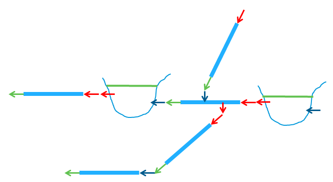
The below figure illustrates the approach: Each light blue element is a model block, and the manipulated flows are shown as red arrows, the output from each model is shown in green and uncontrolled boundaries are displayed as dark blue arrows. A controlled outflow from a reach or a reservoir can be linked to a controlled inflow to another reach or reservoir. An output from a reach (the outflow) can be linked to a boundary inflow of another reach or reservoir.

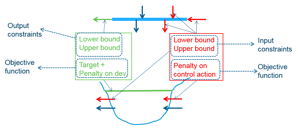
Once configured, each model block provides the global optimisation model with a contribution to the objective function and definition of constraints, see the below figure. This modular approach builds on the following similarities between model blocks: A model block has manipulated flows(also termed control actions), uncontrolled boundaries and model outputs.

• The target for the output provides the contribution to the objective function, and so does a penalty on the the control action.
• The lower and upper bounds on the output define the output constraints.
• The lower and upper bounds on the inputs define the input constraints.

Though the underlying linear models are different, the model blocks for a reach and for a reservoir have similar properties: input (manipulated flow), uncontrolled boundaries and model output.

The reach block provides a simple time delay model. The outflow is obtained by shifting the inflow in time, i.e. the shape of the hydrograph is not changed. This reach model does not model storage in the reach. A reach can have multiple lateral flows (both inflows and outflows) and these may be point sources or distributed along all or a part of the reach. The output variable of a reach is the outflow (in m³/s), which sums up the contributions from all (delayed) in- and outflows along the reach.

The reservoir block calculates a mass balance: the change in volume equals the difference between inflows and outflows. Two formulations are available: the first assumes vertical sides of the reservoir; in this approach, a certain volume change will always imply the same level change no matter the initial level. The second handles a non-linear level-volume relation; internally this approach uses “volume” as state variable, but before presenting the results, the volumes are converted to levels.

List of available model blocks

• Reach
• Reservoir (volume)
  • Uses volume as state variable
  • Initial value, bounds and reference values for the output must be specified as volumes, too.
• Reservoir (level-volume)
  • Uses volume as state variable
  • Initial value, bounds and reference values for the output are specified as levels
  • A level-volume curve must be specified, this will be used to convert the specified levels to volumes prior to the calculation, and to convert output volumes to levels for the results
• Reservoir (level)
  • Uses level as state variable
  • Instead of a level-volume curve, the surface area must be specified
• Reservoir with overflow (volume)
  • As “Reservoir (volume)”, but all water that would make the volume exceed the upper bound will be removed and quantified as overflow
• Reservoir with overflow (level-volume)
  • As “Reservoir (level-volume)”, but all water that would make the volume exceed the upper bound will be removed and quantified as overflow
• Linear reservoir
  • Linear relation between outflow and volume
  • Uses outflow as state variable

Optimisation

The constraints

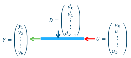
When a block (say a reach) is configured, the data input is interpreted by the MPC, which sets up the optimisation “behind the scenes”. Now, have a look at the reach block in the below figure, which shows a single reach, where manipulated flow (U), output (Y) and uncontrolled boundaries (D) have been indicated for a forecast of k time steps.

Each of these quantities takes a specific value at every time step during the forecast – this is visualised by the vectors in the above figure. Imagine a controlled forecast of 7 days length with hourly time steps. This gives in total $7 \cdot 24 = 168$ time steps in each of which the optimisation has to determine the optimal flow $u_i$.

A bound on this decision will result in $168$ constraints (one inequality to be fulfilled in each time step); therefore, upper and lower bounds will result in $2 \cdot 168 = 336$ constraint inequalities.

Likewise, upper and lower bounds on the output will add another $336$ constraint inequalities to the optimisation problem.

The optimisation is formulated as a minimisation of a quadratic program. A quadratic program has a quadratic objective function and linear constraints. This means that the objective function contains terms with squares of the manipulated variables $(u_0,\dots,u_{k-1})$, whereas the constraint inequalities are linear.

For the constraints on the control actions ($u_i$), linearity is readily fulfilled for “simple constraints” that just impose a constant value as upper or lower bound.

For the constraints on the output, the function that maps the effect of the control actions to the outputs must be linear. This requirement is fulfilled both for the mass-balance calculation for the reservoir block and the time delay model for the reach block. The forecast for the full time horizon is made by recursively using the state from the previous time step as initial condition. The recursion results in a general formulation of the output over the forecast horizon as function of the control.

The below figure shows the linear function that maps manipulated flows (a.k.a controls or decisions or inputs) to outputs, taking initial conditions and uncontrolled boundaries into account. $Y$ is the system output at all time steps in the forecast, $x_0$ is the initial state, $U$ is the control input at all time steps. $O$, $G_u$ and $G_d$ are linear operators, that are obtained by recursively calculating the next state from the previous.

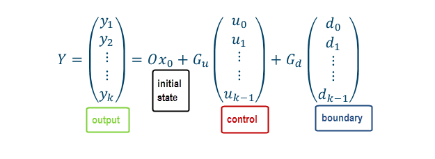
The equation in this figure applies both to a reach block and to a reservoir block. In fact, it applies to any model block, where the state transition is a linear function of the control.

The bounds on the outputs are formulated by setting each output ($y_i$) less or equal to the bounding value (or greater or equal to…). Isolating the terms related to $u_i$ finishes the formulation of the constraint inequalities – and it is obvious that these constraints are linear in $u_i$.

The objective function

Each location with a manipulated flow and each location with an output may contribute to the objective function. For outputs the objectives relate to reaching a target value and not exceeding constraints. For manipulated flows, the objectives relate to reaching a target and make the flow smooth. The objective function aggregates the expressions listed in the next sections into a single number, and the optimisation manipulates the gate/valve/pump flows to minimise this number. The weight/penalty in each expression prioritises how important this particular sub-objective (at this particular location) is, in relation to all other sub-objectives. A high weight puts a higher (relative) importance to a sub-objective.

Minimise deviation from target

Each model block gives a contribution to the objective function that quantifies the output’s deviation from the target value: the squared deviations at each time step are aggregated in a sum:

$$\sum_{i=1}^{k} q_i(y_i - r_i)^2$$

Here $y_i$ is the output at time step $i$, $r_i$ is the target value for time step $i$, and $q_i$ is a weight. The target, $r_i$, may be a constant or vary over the control horizon. The weight, q_i, will in many cases be constant over the forecast horizon, but an option exist to specify it as time varying.

Minimise violation of constraints

The constraint inequalities, which are set up (for each time step) for lower and upper bounds on control actions (manipulated flows) and outputs (outflows and reservoir levels), are so-called hard constraints.

A hard constraint cannot be violated by the optimisation. Therefore, if violation (in the real world) is unavoidable, then the hard-constrained optimisation will have “no feasible solutions”. In the flood protection application an example of unavoidable violation of the constraints could be a desired maximum flow constraint on the channel flow downstream of a regulator. If the natural inflows are large, this “operational goal of not exceeding a certain flow” cannot be fulfilled, even not with no release from the regulator at all.

Therefore, a mechanism that allows violation of (some) constraints is needed. Constraints that can be violated are termed soft constraints, and the violation is penalised by adding an extra term to the objective function.

$$\sum_{i=1}^{k}ps_i^2$$

Here $s_i$ denotes the exceedance (in case of upper bounds) and the undershot (in case of lower bounds). $s_i$ is also known as a slack variable. The violation penalty, $p$, is constant over the forecast horizon.

Currently, soft constraints can only be defined for outputs.

Minimise the control action

The "control action" is the "flow through a control structure", e.g. the flow through a gate, valve or pump. This objective can be used to make the manipulated flow stick to a target, and if no target is specified "zero flow" is the default target. The default target of zero flow should only be used, if it is an operational goal to hold back the water upstream of the controllable device as long as possible. In many cases the goal is rather to stabilise the flow, i.e. avoid too sudden changes. In that case the objective "Smooth the control action" should be used.

$$\sum_{i=0}^{k-1} \sigma_i(u_i-r_i)^2$$

Here $u_i$ is the control action (the manipulated flow) at time step $i$, $\sigma_i$ is a weight/penalty on deviating from the target and $r_i$ is a value for the manipulated flow. Both penalty and target may be constant or time varying.

Smooth the control action

This objective puts a penalty ($\sigma$ on the manipulated flow ($u_i$) if it deviates from the flow in the previous time step ($u_{i-1}$). $\sigma$ is constant over the time horizon. The aim is to dampen changes in the manipulated flow, so as to avoid too sudden jumps in the control.

$$\sum_{i=0}^{k-1} \sigma(u_i-u_{i-1})^2$$

As the sum starts at $i = 0$, the very first term in the sum needs $u_{-1}$, i.e. the manipulated flow from the time step prior to starting the optimisation. This ensures that there is a cost related to making a change in the manipulated flow also in the very first time step.

Debugging infeasibility

On some occasions, the optimisation problem does not have a solution, and is said to be infeasible. This occurs when some of the constraints contradict each other so they cannot all be fulfilled. A simple example of constraints in contradiction is if a reservoir is required both to have a level above 2 m and below 1 m, which obviously cannot be achieved at the same time.

For MPC's optimisation set up for a water network, the conflicting constraints can be harder to identify, because the optimisation problem encapsulates the dynamic development of the system (as function of the manipulated variables) for the entire prediction horizon. This means that the violation of a constraint (e.g. a maximum water level) can happen at some time during the prediction horizon, but it is likely caused by the constraint on a manipulated variable. The optimisation has full information about the dynamics within the prediction horizon, so if the optimisation reports "infeasibility" it means that no combination of the manipulated variables (which for instance could be the flow rate (at each time step) of the release from the reservoir) can satisfy the constraints. In the above case of a reservoir with an MPC-manipulated release, an infeasible situation can occur if there is also defined a maximum flow rate for the reservoir release - and this flow rate, even if used from the very first time step, cannot empty the reservoir fast enough to make it stay below the required maximum level.

Usually the constraints on the manipulated variables are rooted in physical limitations, for instance a minimum discharge for a manipulated flow. The minimum discharge is often "zero", corresponding to a closed gate, and if the water cannot go back upstream through the gate, it does not make sense to allow negative values for the release as this cannot be realised by the physical system. The constraints on the system state are often expressing a "desired operating range", which in some cased might be violated - it might even be impossible to avoid violation i the physical system. An example is a maximum desired flow rate at a reach outflow. The maximum flow might be violated if the uncontrolled inflows to the reach (upstream of the reach otflow) exceed the specified maximum flow. Even by closing all controlled flows, it is not possible to stay under the limit.

The following subsections outline a number of common cases that cause infeasibility, and explains how to get a log from the optimisation solver with an infeasibility report, and how this report should be interpreted. It is important to understand that most infeasibilities occur due to a combination of requirements to the state of the system and requirements to the manipulated variables. The state of the system are water levels or volumes of reservoirs or outflows from reaches, and the manipulated variables are the flow rates that MPC has been given to optimise. MPC's optimisation adresses manipulation of flow rates at all time stamps within the prediction horizon in order to obtain/maintain the desired reservoir levels/volumes and reach outflows at all time stamps within the prediction horizon.

The below examples are constructed to be infeasible. For each example, the cause of the infeasibility is explained up front, and then we walk through the infeasibility report from the log to learn how the different causes of infeasibility are reported.

Print solver log

This instruction on how to activate writing of the log assumes that mosek is used as optimisation solver. If MPC is invoked from MIKE OPERATIONS, the solver class DHI.ConvexOptimization.Mosek.SolverQP is called from a python script. Activation of writing of mosek's log, and a path to direct it to can optionally be given as input arguments when instantiating SolverQP. If no arguments are specified, no log is written.

import clr #access to MPC-libraries, which are specified below
clr.AddReference('DHI.ConvexOptimization.Mosek')
from DHI.ConvexOptimization.Mosek import *

loggingDirectory = 'C:\mylogs'
solver = SolverQP(writeLog=True, logDir=loggingDirectory, writeProblem=False)

The above call will direct mosek's log to the directory C:\mylogs - the name is automated and contains the timestamp in the format "yyyy-MM-dd_HH-mm-ss.ff", for instance "mosek_2023-02-24_18-54-26.44.log". The accuracy of the time stamp is set to 1/100 s, so optimisations initiated within the time range of a second do not interfere with each other's logs. This is rarely the case in real-time systems, but on desktop simulations (as well as in unit testing) optimisations might be launched in a straight sequence.

If writeLog=True, but no logDir is specified, the log by default goes to %LOCALAPPDATA%\mosek.

If writeProblem=True, the optimisation problem is dumped to a json file in the logDir. Only writing of the log is needed for debugging infeasibility.

Max flow causes infeasible reservoir level

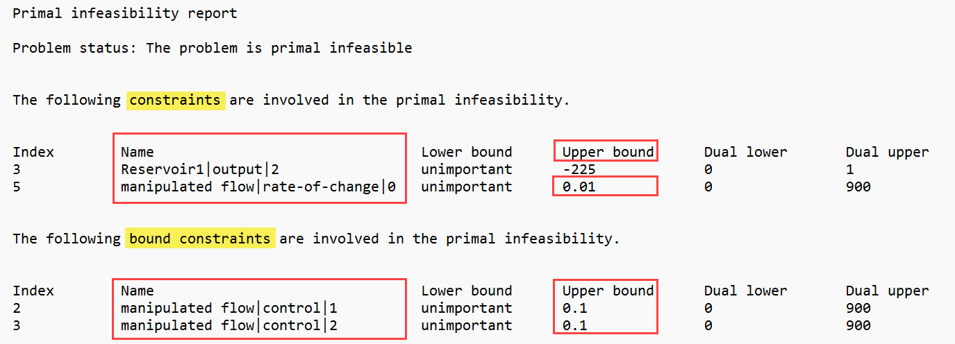
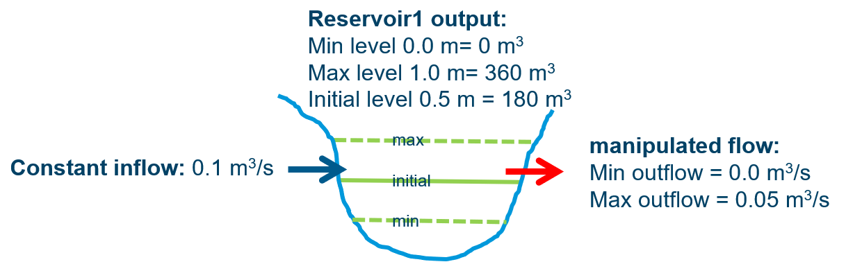In an optimisation set up with 15 min time step, the above reservoir will reach the max level (1 m) after two time steps, even if the manipulated flow runs at max flow rate (0.05 m3/s), because the net inflow to the reservoir cannot get below 0.1-0.05 = 0.05 m3/s. The infeasibility report in the log is shown below:

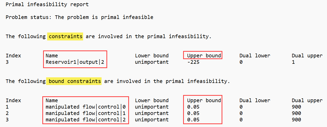
The log is divided in two parts, the first regards "constraints" and the second regards "bound constraints". Roughly speaking, the "constraints" section points out the infeasible system state, and the "bound constraints" section points out the manipulated varible, whose constraints leads to violation of the system state constraint (an exception to this occurs for rate-of-change constraints on the manipulated flow, which will appear in the "constraints" section).

In the "constraints" section, the "Name" column shows "Reservoir1|output|2". This tells that the reservoir named "Reservoir1" in the setup reaches a limit on its "output" at time index "2". Inspecting the columns "Lower bound" and "Upper bound", we find that the lower bound is "unimportant", so the violation is of the upper bound (i.e. the max level of the reservoir). The numbers in these two columns do not have a direct interpretation, as they are processed to take the system dynamics into account. So a maximum level of 1 m does not show as "1" in this column.

The time index is zero-based (i.e. first time step has index=0), so it is at the third time step that the reservoir level becomes infeasible. This does not indicate that the third time step is the only time step where a solution that satisfies all constraints cannot be found, the third time step is just the first point in time where it becomes apparent that no matter how the manipulated flow is chosen in all previous time steps, it is not possible to fulfill all constraints (both those on the reservoir level and those on the manipulated flow).

The limiting constraint on the manipulated flow is reported on in the "bound constraints" section. Under "bound constraints", the name column shows three entries, all related to "manipulated flow|control|some_index". This tells that it the MPC-controlled flow "manipulated flow", which reaches its limit in the first three time steps (index 0, 1, 2). The column "Lower bound" says "unimportant", so it is the upper bound that reaches the limit. As opposed to the "constraints" section, the numbers in the "Upper bound" of the "bound constraints section" correspond directly to the specified maximum flow.

Summing up: the optimisation is infeasible, because the upper bound on "manipulated flow" does not allow a release, which is large enough to avoid exceeding the maximum level of "Reservoir1". The infeasibility tracks all the way back to the first time step, because of the upper bound on "manipulated flow".

Max rate-of-change causes infeasible reservoir level

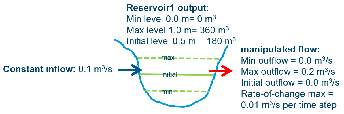The setup from the previous section is changed a bit, so the max outflow is increased to 0.2 m3/s. So if "manipulated flow" runs at max, the level in "Reservoir1" will stay below the maximum level. However, we have added a constraint on how fast "manipulated flow" is allowed to change, and this is (for sake of the example) set very low - "manipulated flow" can at max change by 0.01 m3/s from one time setp to the next. When a rate-of-change constraint is included, the initial value of "manipulated flow" becomes interesting - in this case it is set to zero, which means that given the maximum rate of change, there is no way the optimisation can turn up the flow to 0.2 m3/s in a few time steps.

The log reads: 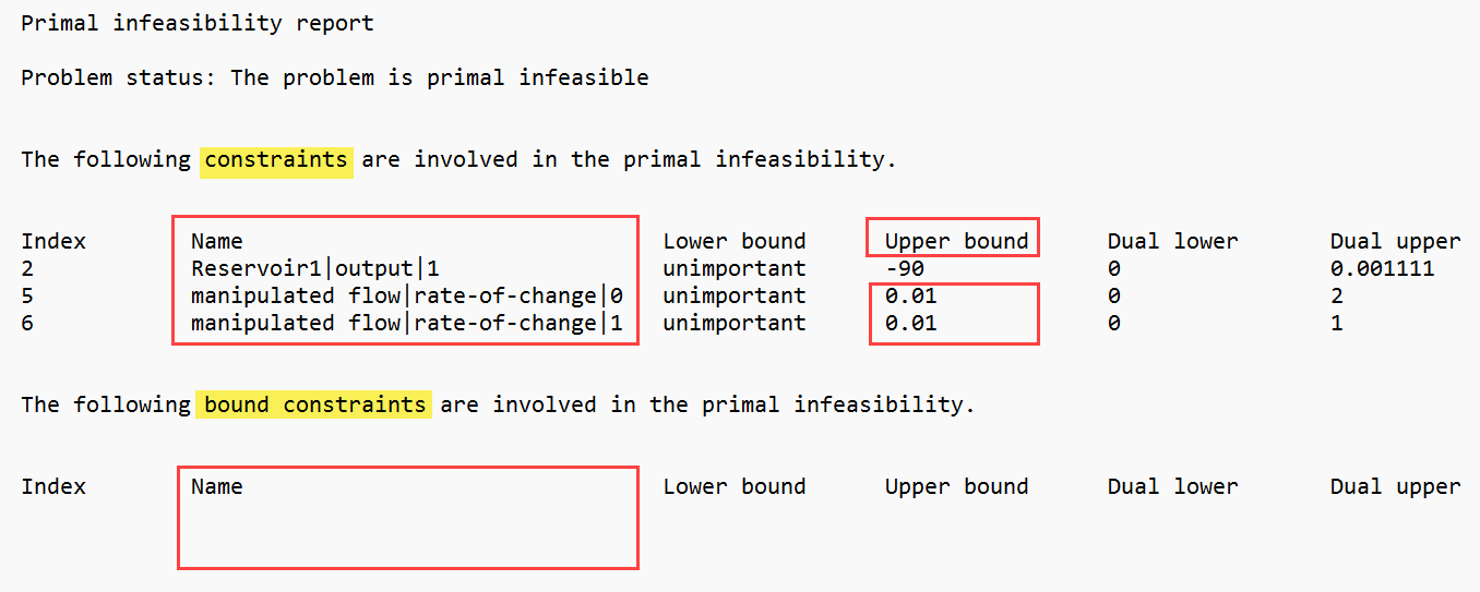The log shows that the level of "Reservoir1" reaches its upper bound already in the second time step (index 1) and that this is caused by the upper bound on the rate-of-change on "manipulated flow" starting at the first time step. The values in the "Upper bound" column (0.01)corresponds to the maximum rate of change (in m3/s) per time step (in seconds).

The log does not show that the rate-of-change constraint on "manipulated flow" becomes a limiting factor only because "manipulated flow" starts out at zero. When a rate-of-change violation is reported, one must check the initial value of the flow in question by hand.

The reason that rate-of-change constraints are reported in the "constraints" section and not in the "bound constraints" section is that the rate-of-change is calculated as the flow at the current time step minus the flow at the previous time step. Seen from the optimiser's point of view, this is a constraint on a function of the manipulated variables and not directly on manipulated variables. Therefore, rate-of-change constraints appear in the same section as the other system states (which are all functions of the manipulated variables).

The "bound constraints" section is empty, which means that neither lower nor upper limit on "manipulated flow" becomes a limiting factor.

Summing up: The uptimisation is infeasible, because the upper bound on the rate-of-change on "manipulated flow" prevents it to rise (from zero) to a value that can empty "Reservoir1" before it runs full. The max on "manipulated flow"is not a limiting factor.

Infeasible reservoir level caused by ?

Consider the previous setup, but with a slight change: The maximum of "manipulated flow" is decreased from 0.2 m3/s to 0.1 m3/s. If "manipulated flow" runs at max, it would balance the inflow, and the level of "Reservoir1" stays below max. However, the rate-of-change constraint on "manipulated flow" prevents it to rise quickly enough to avoid filling "Reservoir1" to max level.

The log reads: The infeasibility report for this setup points to "manipulated flow"'s rate-of-change in the first time step and to "manipulated flow"'s upper bound in the next two time steps. This may be interpreted as "if the first time step had allowed a larger increase of "manipulated flow", then the upper bound on "manipulated flow" would become the limiting factor. Still, the main cause of the infeasibility is the rate-of-change constraint (in combination with the zero initial flow).

Summing up: When a rate-of-change constraint for a single time step is included in the infeasibility report, it is likely that this constraint is is acutally limiting more than just this time step.

Infeasible initial condition for a reservoir

Another situation which can cause either rate-of-change or a bound on a manipulated flow to appear in the infeasibility report is if the initial level (or volume) of a reservoir is outside of the bounds. If either the rate-of-change bound or the bound on the manipulated flow itself prevents the reservoir level to get inside the bounds in the first time step, infeasibility occurs. The entries in the infeasibility report will all point to index "0" as already the first time step becomes infeasible.

Uncertainty

At present the support for uncertain boundary conditions is an experimental feature. The method is an ensemble approach, where an ensemble can be specified for the boundary time series. The resulting optimised control actions is not an ensemble – the optimised control actions are “the best choice, taking all realisations of the boundary conditions into account”.

In this experimental implementation, the boundary condition specified as the first ensemble member is pulled forward when running a closed-loop simulation where the surrogate model itself is used for evaluation. This corresponds to assuming that the first member of the ensemble forecast was actually realised. Therefore, the ensemble member with the highest probability should be put as the first member in the boundary time series.

Configuration.EnsembleSize determines the number of members in the ensemble. Not setting this property will result in a deterministic simulation (with ensemble size = 1). A probability can be assigned to each member by Configuration.RealisationProbability. If Configuration.RealisationProbability is left out, all realisations will have equal probability assigned.

Having set Configuration.EnsembleSize to a number greater than one, requires at least some of the boundary time series to be ensemble time series. These time series must contain a number of members, which equals the ensemble size. Still, some of the boundary time series are allowed to be deterministic. During the optimisation, these will be duplicated to the distinct realisations.

Comments and hints

Set up each block (in this case each reservoir and each reach) in a separate configuration script. Such a script must return the data records needed for connecting the blocks. For reaches, this will be InflowData, maybe LateralInflowData and LateralOutflowData, and the ReachData record itself. For reservoirs, return item candidates are InflowData, OutflowData and ReservoirData.

Flows that are marked mpcControlled will be treated as such only when an optimisation run is employed. When running uncontrolled simulations, the mpcControlled flag will determine whether a specified flow is represented as a manipulated input flow (mpcControlled = True) or as an uncontrolled boundary (mpcControlled = False) in the surrogate model equations. In both cases, the time series specified for the flow needs to cover the simulation period, and the final result does not depend on how the flow was represented in the simulation.

Calibrate each block separately. This is possible if simulation data from a high-fidelity model (i.e. MIKE 11) are available.

Long delay times for the reaches are memory consuming. This can be remedied by splitting a long reach into smaller parts. Guidelines for the choice of splitting points are:

• If the lateral flows along the river belong to “different sections”, then split
• Split at points where measured data are available
• Split at points that will be subject to constraint (a constraint on an “inline flow” must be formulated as a constraint on the outflow from a reach – therefore a split at all constrained points is needed)
• The water travels faster the steeper the channel is – so if the steepness changes, then split.

On the other hand, reaches should not be too short either. The surrogate model has an inherent delay of one time step, so for a simulation the first output has a time stamp, which is one time step later than simulation start. A reach should at minimum have a delay of one time step.

When connecting blocks into a network, remember:

• If one or both flows in a connection are marked mpcControlled, then the connection will be controlled, and the control will always be exerted on the “source flow” (i.e. the upstream of the two flows in the connection)
• The outflow from a reach cannot be controlled, as the reach model does not allow storage in the reach. If a reach is connected to a controlled inflow, then the mpcControlled = True flag is ignored, and the flow through the connection will end up being uncontrolled.

Terminology

Manipulated variables, Input, controls, control actions, decisions, forcings, optimisation variables, are all names of the quantities we want to control, and which are subject to optimisation.

State variables are the “internal model variables”.

Output, model output, are names of the quantities that we can set targets for and restrict by output constraints. The model output is a linear combination of the state variables, the simplest being a one-to-one correspondence: all state variables are mapped directly to output variables. In practice, only a subset of the state variables make their way to the output.

Results are derived from the output. The results may be a non-linear function of the outputs (like the level-volume relation for a reservoir). The important thing is that the non-linearity does not enter the MPC calculation, as the conversion from output to results is a post-processing.

Target value, reference value . This is the desired value of the output of a block, the value that the optimisation will work on attaining.

Boundaries, disturbances. These are impacts on the system that we cannot control – but through the controls we can counteract their effects.